ENGR 1330 Computational Thinking with Data Science

Last GitHub Commit Date: 31 January 2021

Lesson 8 The Pandas module

• How to install
  • Anaconda
  • JupyterHub/Lab (on Linux)
  • JupyterHub/Lab (on MacOS)
  • JupyterHub/Lab (on Windoze)
• About Pandas
  • Arrays
    • ...
    • ...
  • Array Methods

---

Special Script Blocks

%%html
<!--Script block to left align Markdown Tables-->
<style>
  table {margin-left: 0 !important;}
</style>

---

Objectives

1. To understand the dataframe abstraction as implemented in the Pandas library(module).
   1. To be able to access and manipulate data within a dataframe
   2. To be able to obtain basic statistical measures of data within a dataframe
2. Read/Write from/to files
   1. MS Excel-type files (.xls,.xlsx,.csv) (LibreOffice files use the MS .xml standard)
   2. Ordinary ASCII (.txt) files
3. Access files directly from a URL (advanced concept)
   1. Using a wget-type function
   2. Using a curl-type function
   3. Using API keys (future versions)

Pandas:

Pandas is the core library for dataframe manipulation in Python. It provides a high-performance multidimensional array object, and tools for working with these arrays. The library’s name is derived from the term ‘Panel Data’. If you are curious about Pandas, this cheat sheet is recommended: https://pandas.pydata.org/Pandas_Cheat_Sheet.pdf

Data Structure

The Primary data structure is called a dataframe. It is an abstraction where data are represented as a 2-dimensional mutable and heterogenous tabular data structure; much like a Worksheet in MS Excel. The structure itself is popular among statisticians and data scientists and business executives.

According to the marketing department "Pandas Provides rich data structures and functions designed to make working with data fast, easy, and expressive. It is useful in data manipulation, cleaning, and analysis; Pandas excels in performance and productivity "

---

The Dataframe

A data table is called a DataFrame in pandas (and other programming environments too). The figure below from https://pandas.pydata.org/docs/getting_started/index.html illustrates a dataframe model:

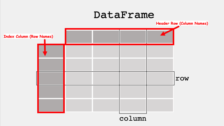
Each column and each row in a dataframe is called a series, the header row, and index column are special. Like MS Excel we can query the dataframe to find the contents of a particular cell using its row name and column name, or operate on entire rows and columns

To use pandas, we need to import the module.

Computational Thinking Concepts

The CT concepts expressed within Pandas include:

• Decomposition : Data interpretation, manipulation, and analysis of Pandas dataframes is an act of decomposition -- although the dataframes can be quite complex.
• Abstraction : The dataframe is a data representation abstraction that allows for placeholder operations, later substituted with specific contents for a problem; enhances reuse and readability. We leverage the principle of algebraic replacement using these abstractions.
• Algorithms : Data interpretation, manipulation, and analysis of dataframes are generally implemented as part of a supervisory algorithm.

Module Set-Up

In principle, Pandas should be available in a default Anaconda install

• You should not have to do any extra installation steps to install the library in Python
• You do have to import the library in your scripts

How to check

• Simply open a code cell and run import pandas if the notebook does not protest (i.e. pink block of error), the youis good to go.

import pandas

If you do get an error, that means that you will have to install using conda or pip; you are on-your-own here! On the content server the process is:

1. Open a new terminal from the launcher
2. Change to root user su then enter the root password
3. sudo -H /opt/jupyterhib/bin/python3 -m pip install pandas
4. Wait until the install is complete; for security, user compthink is not in the sudo group
5. Verify the install by trying to execute import pandas as above.

The process above will be similar on a Macintosh, or Windows if you did not use an Anaconda distribution. Best is to have a sucessful anaconda install, or go to the GoodJobUntilMyOrgansGetHarvested.

If you have to do this kind of install, you will have to do some reading, some references I find useful are:

1. https://jupyterlab.readthedocs.io/en/stable/user/extensions.html
2. https://www.pugetsystems.com/labs/hpc/Note-How-To-Install-JupyterHub-on-a-Local-Server-1673/#InstallJupyterHub
3. https://jupyterhub.readthedocs.io/en/stable/installation-guide-hard.html (This is the approach on the content server which has a functioning JupyterHub)

Dataframe-type Structure using primative python

First lets construct a dataframe like object using python primatives. We will construct 3 lists, one for row names, one for column names, and one for the content.

import numpy
mytabular = numpy.random.randint(1,100,(5,4))
myrowname = ['A','B','C','D','E']
mycolname = ['W','X','Y','Z']
mytable = [['' for jcol in range(len(mycolname)+1)] for irow in range(len(myrowname)+1)] #non-null destination matrix, note the implied loop construction

The above builds a placeholder named mytable for the psuedo-dataframe. Next we populate the table, using a for loop to write the column names in the first row, row names in the first column, and the table fill for the rest of the table.

for irow in range(1,len(myrowname)+1): # write the row names
    mytable[irow][0]=myrowname[irow-1]
for jcol in range(1,len(mycolname)+1): # write the column names
    mytable[0][jcol]=mycolname[jcol-1]  
for irow in range(1,len(myrowname)+1): # fill the table (note the nested loop)
    for jcol in range(1,len(mycolname)+1):
        mytable[irow][jcol]=mytabular[irow-1][jcol-1]

Now lets print the table out by row and we see we have a very dataframe-like structure

for irow in range(0,len(myrowname)+1):
    print(mytable[irow][0:len(mycolname)+1])

['', 'W', 'X', 'Y', 'Z']
['A', 3, 78, 15, 62]
['B', 82, 5, 27, 80]
['C', 36, 35, 63, 30]
['D', 88, 77, 55, 74]
['E', 9, 86, 44, 87]

We can also query by row

print(mytable[3][0:len(mycolname)+1])

['C', 36, 35, 63, 30]

Or by column

for irow in range(0,len(myrowname)+1):  #cannot use implied loop in a column slice
    print(mytable[irow][2])

X
78
5
35
77
86

Or by row+column index; sort of looks like a spreadsheet syntax.

print(' ',mytable[0][3])
print(mytable[3][0],mytable[3][3])

  Y
C 63

Now we shall create a proper dataframe

We will now do the same using pandas

mydf = pandas.DataFrame(numpy.random.randint(1,100,(5,4)), ['A','B','C','D','E'], ['W','X','Y','Z'])
mydf

	W	X	Y	Z
A	33	46	69	49
B	65	66	90	24
C	91	63	19	69
D	83	24	96	95
E	75	23	71	74

We can also turn our table into a dataframe, notice how the constructor adds header row and index column

mydf1 = pandas.DataFrame(mytable)
mydf1

	0	1	2	3	4
0		W	X	Y	Z
1	A	3	78	15	62
2	B	82	5	27	80
3	C	36	35	63	30
4	D	88	77	55	74
5	E	9	86	44	87

To get proper behavior, we can just reuse our original objects

mydf2 = pandas.DataFrame(mytabular,myrowname,mycolname)
mydf2

	W	X	Y	Z
A	3	78	15	62
B	82	5	27	80
C	36	35	63	30
D	88	77	55	74
E	9	86	44	87

Why are mydf and mydf2 different?

Getting the shape of dataframes

The shape method, which is available after the dataframe is constructed, will return the row and column rank (count) of a dataframe.

mydf.shape

(5, 4)

mydf1.shape

(6, 5)

mydf2.shape

(5, 4)

Appending new columns

To append a column simply assign a value to a new column name to the dataframe

mydf['new']= 'NA'

mydf

	W	X	Y	Z	new
A	33	46	69	49	NA
B	65	66	90	24	NA
C	91	63	19	69	NA
D	83	24	96	95	NA
E	75	23	71	74	NA

Appending new rows

This is sometimes a bit trickier but here is one way:

• create a copy of a row, give it a new name.
• concatenate it back into the dataframe.

newrow = mydf.loc[['E']].rename(index={"E": "X"}) # create a single row, rename the index
newtable = pandas.concat([mydf,newrow]) # concatenate the row to bottom of df - note the syntax

newtable

	W	X	Y	Z	new
A	33	46	69	49	NA
B	65	66	90	24	NA
C	91	63	19	69	NA
D	83	24	96	95	NA
E	75	23	71	74	NA
X	75	23	71	74	NA

Removing Rows and Columns

To remove a column is straightforward, we use the drop method

newtable.drop('new', axis=1, inplace = True)
newtable

	W	X	Y	Z
A	33	46	69	49
B	65	66	90	24
C	91	63	19	69
D	83	24	96	95
E	75	23	71	74
X	75	23	71	74

To remove a row, you really got to want to, easiest is probablty to create a new dataframe with the row removed

newtable = newtable.loc[['A','B','D','E','X']] # select all rows except C
newtable

	W	X	Y	Z
A	33	46	69	49
B	65	66	90	24
D	83	24	96	95
E	75	23	71	74
X	75	23	71	74

# or just use drop with axis specify
newtable.drop('X', axis=0, inplace = True)

newtable

	W	X	Y	Z
A	33	46	69	49
B	65	66	90	24
D	83	24	96	95
E	75	23	71	74

Indexing

We have already been indexing, but a few examples follow:

newtable['X'] #Selecing a single column

A    46
B    66
D    24
E    23
Name: X, dtype: int64

newtable[['X','W']] #Selecing a multiple columns

	X	W
A	46	33
B	66	65
D	24	83
E	23	75

newtable.loc['E'] #Selecing rows based on label via loc[ ] indexer

W    75
X    23
Y    71
Z    74
Name: E, dtype: int64

newtable
    

	W	X	Y	Z
A	33	46	69	49
B	65	66	90	24
D	83	24	96	95
E	75	23	71	74

newtable.loc[['E','D','B']] #Selecing multiple rows based on label via loc[ ] indexer

	W	X	Y	Z
E	75	23	71	74
D	83	24	96	95
B	65	66	90	24

newtable.loc[['B','E','D'],['X','Y']] #Selecting elements via both rows and columns via loc[ ] indexer

	X	Y
B	66	90
E	23	71
D	24	96

Conditional Selection

mydf = pandas.DataFrame({'col1':[1,2,3,4,5,6,7,8],
                   'col2':[444,555,666,444,666,111,222,222],
                   'col3':['orange','apple','grape','mango','jackfruit','watermelon','banana','peach']})
mydf

	col1	col2	col3
0	1	444	orange
1	2	555	apple
2	3	666	grape
3	4	444	mango
4	5	666	jackfruit
5	6	111	watermelon
6	7	222	banana
7	8	222	peach

#What fruit corresponds to the number 555 in ‘col2’?

mydf[mydf['col2']==555]['col3']

1    apple
Name: col3, dtype: object

#What fruit corresponds to the minimum number in ‘col2’?

mydf[mydf['col2']==mydf['col2'].min()]['col3']

5    watermelon
Name: col3, dtype: object

Descriptor Functions

#Creating a dataframe from a dictionary

mydf = pandas.DataFrame({'col1':[1,2,3,4,5,6,7,8],
                   'col2':[444,555,666,444,666,111,222,222],
                   'col3':['orange','apple','grape','mango','jackfruit','watermelon','banana','peach']})
mydf

	col1	col2	col3
0	1	444	orange
1	2	555	apple
2	3	666	grape
3	4	444	mango
4	5	666	jackfruit
5	6	111	watermelon
6	7	222	banana
7	8	222	peach

head method

Returns the first few rows, useful to infer structure

#Returns only the first five rows

mydf.head()

	col1	col2	col3
0	1	444	orange
1	2	555	apple
2	3	666	grape
3	4	444	mango
4	5	666	jackfruit

info method

Returns the data model (data column count, names, data types)

#Info about the dataframe

mydf.info()

<class 'pandas.core.frame.DataFrame'>
RangeIndex: 8 entries, 0 to 7
Data columns (total 3 columns):
 #   Column  Non-Null Count  Dtype 
---  ------  --------------  ----- 
 0   col1    8 non-null      int64 
 1   col2    8 non-null      int64 
 2   col3    8 non-null      object
dtypes: int64(2), object(1)
memory usage: 320.0+ bytes

describe method

Returns summary statistics of each numeric column.
Also returns the minimum and maximum value in each column, and the IQR (Interquartile Range).
Again useful to understand structure of the columns.

#Statistics of the dataframe

mydf.describe()

	col1	col2
count	8.00000	8.0000
mean	4.50000	416.2500
std	2.44949	211.8576
min	1.00000	111.0000
25%	2.75000	222.0000
50%	4.50000	444.0000
75%	6.25000	582.7500
max	8.00000	666.0000

Counting and Sum methods

There are also methods for counts and sums by specific columns

mydf['col2'].sum() #Sum of a specified column

3330

The unique method returns a list of unique values (filters out duplicates in the list, underlying dataframe is preserved)

mydf['col2'].unique() #Returns the list of unique values along the indexed column 

array([444, 555, 666, 111, 222])

The nunique method returns a count of unique values

mydf['col2'].nunique() #Returns the total number of unique values along the indexed column 

5

The value_counts() method returns the count of each unique value (kind of like a histogram, but each value is the bin)

mydf['col2'].value_counts()  #Returns the number of occurences of each unique value

666    2
444    2
222    2
555    1
111    1
Name: col2, dtype: int64

Using functions in dataframes - symbolic apply

The power of Pandas is an ability to apply a function to each element of a dataframe series (or a whole frame) by a technique called symbolic (or synthetic programming) application of the function.

This employs principles of pattern matching, abstraction, and algorithm development; a holy trinity of Computational Thinning.

It's somewhat complicated but quite handy, best shown by an example:

def times2(x):  # A prototype function to scalar multiply an object x by 2
    return(x*2)

print(mydf)
print('Apply the times2 function to col2')
mydf['col2'].apply(times2) #Symbolic apply the function to each element of column col2, result is another dataframe

   col1  col2        col3
0     1   444      orange
1     2   555       apple
2     3   666       grape
3     4   444       mango
4     5   666   jackfruit
5     6   111  watermelon
6     7   222      banana
7     8   222       peach
Apply the times2 function to col2

0     888
1    1110
2    1332
3     888
4    1332
5     222
6     444
7     444
Name: col2, dtype: int64

Sorts

mydf.sort_values('col2', ascending = True) #Sorting based on columns 

	col1	col2	col3
5	6	111	watermelon
6	7	222	banana
7	8	222	peach
0	1	444	orange
3	4	444	mango
1	2	555	apple
2	3	666	grape
4	5	666	jackfruit

mydf.sort_values('col3', ascending = True) #Lexiographic sort

	col1	col2	col3
1	2	555	apple
6	7	222	banana
2	3	666	grape
4	5	666	jackfruit
3	4	444	mango
0	1	444	orange
7	8	222	peach
5	6	111	watermelon

Aggregating (Grouping Values) dataframe contents

#Creating a dataframe from a dictionary

data = {
    'key' : ['A', 'B', 'C', 'A', 'B', 'C'],
    'data1' : [1, 2, 3, 4, 5, 6],
    'data2' : [10, 11, 12, 13, 14, 15],
    'data3' : [20, 21, 22, 13, 24, 25]
}

mydf1 = pandas.DataFrame(data)
mydf1

	key	data1	data2	data3
0	A	1	10	20
1	B	2	11	21
2	C	3	12	22
3	A	4	13	13
4	B	5	14	24
5	C	6	15	25

# Grouping and summing values in all the columns based on the column 'key'

mydf1.groupby('key').sum()

	data1	data2	data3
key
A	5	23	33
B	7	25	45
C	9	27	47

# Grouping and summing values in the selected columns based on the column 'key'

mydf1.groupby('key')[['data1', 'data2']].sum()

	data1	data2
key
A	5	23
B	7	25
C	9	27

Filtering out missing values

Filtering and cleaning are often used to describe the process where data that does not support a narrative is removed ;typically for maintenance of profit applications, if the data are actually missing that is common situation where cleaning is justified.

#Creating a dataframe from a dictionary

df = pandas.DataFrame({'col1':[1,2,3,4,None,6,7,None],
                   'col2':[444,555,None,444,666,111,None,222],
                   'col3':['orange','apple','grape','mango','jackfruit','watermelon','banana','peach']})
df

	col1	col2	col3
0	1.0	444.0	orange
1	2.0	555.0	apple
2	3.0	NaN	grape
3	4.0	444.0	mango
4	NaN	666.0	jackfruit
5	6.0	111.0	watermelon
6	7.0	NaN	banana
7	NaN	222.0	peach

Below we drop any row that contains a NaN code.

df_dropped = df.dropna()
df_dropped

	col1	col2	col3
0	1.0	444.0	orange
1	2.0	555.0	apple
3	4.0	444.0	mango
5	6.0	111.0	watermelon

Below we replace NaN codes with some value, in this case 0

df_filled1 = df.fillna(0)
df_filled1

	col1	col2	col3
0	1.0	444.0	orange
1	2.0	555.0	apple
2	3.0	0.0	grape
3	4.0	444.0	mango
4	0.0	666.0	jackfruit
5	6.0	111.0	watermelon
6	7.0	0.0	banana
7	0.0	222.0	peach

Below we replace NaN codes with some value, in this case the mean value of of the column in which the missing value code resides.

df_filled2 = df.fillna(df.mean())
df_filled2

	col1	col2	col3
0	1.000000	444.0	orange
1	2.000000	555.0	apple
2	3.000000	407.0	grape
3	4.000000	444.0	mango
4	3.833333	666.0	jackfruit
5	6.000000	111.0	watermelon
6	7.000000	407.0	banana
7	3.833333	222.0	peach

---

Reading a File into a Dataframe

Pandas has methods to read common file types, such as csv,xlsx, and json.
Ordinary text files are also quite manageable.

On a machine you control you can write script to retrieve files from the internet and process them.

readfilecsv = pandas.read_csv('CSV_ReadingFile.csv')  #Reading a .csv file
print(readfilecsv)

    a   b   c   d
0   0   1   2   3
1   4   5   6   7
2   8   9  10  11
3  12  13  14  15

Similar to reading and writing .csv files, you can also read and write .xslx files as below (useful to know this)

readfileexcel = pandas.read_excel('Excel_ReadingFile.xlsx', sheet_name='Sheet1') #Reading a .xlsx file
print(readfileexcel)

   Unnamed: 0   a   b   c   d
0           0   0   1   2   3
1           1   4   5   6   7
2           2   8   9  10  11
3           3  12  13  14  15

Writing a dataframe to file

#Creating and writing to a .csv file
readfilecsv = pandas.read_csv('CSV_ReadingFile.csv')
readfilecsv.to_csv('CSV_WritingFile1.csv')
readfilecsv = pandas.read_csv('CSV_WritingFile1.csv')
print(readfilecsv)

   Unnamed: 0   a   b   c   d
0           0   0   1   2   3
1           1   4   5   6   7
2           2   8   9  10  11
3           3  12  13  14  15

#Creating and writing to a .csv file by excluding row labels 
readfilecsv = pandas.read_csv('CSV_ReadingFile.csv')
readfilecsv.to_csv('CSV_WritingFile2.csv', index = False)
readfilecsv = pandas.read_csv('CSV_WritingFile2.csv')
print(readfilecsv)

    a   b   c   d
0   0   1   2   3
1   4   5   6   7
2   8   9  10  11
3  12  13  14  15

#Creating and writing to a .xlsx file
readfileexcel = pandas.read_excel('Excel_ReadingFile.xlsx', sheet_name='Sheet1')
readfileexcel.to_excel('Excel_WritingFile.xlsx', sheet_name='MySheet', index = False)
readfileexcel = pandas.read_excel('Excel_WritingFile.xlsx', sheet_name='MySheet')
print(readfileexcel)

   Unnamed: 0   a   b   c   d
0           0   0   1   2   3
1           1   4   5   6   7
2           2   8   9  10  11
3           3  12  13  14  15

---

References

Overland, B. (2018). Python Without Fear. Addison-Wesley ISBN 978-0-13-468747-6.

Grus, Joel (2015). Data Science from Scratch: First Principles with Python O’Reilly Media. Kindle Edition.

Precord, C. (2010) wxPython 2.8 Application Development Cookbook Packt Publishing Ltd. Birmingham , B27 6PA, UK ISBN 978-1-849511-78-0.

# Preamble script block to identify host, user, and kernel
import sys
! hostname
! whoami
print(sys.executable)
print(sys.version)
print(sys.version_info)

ip-172-26-4-2
compthink
/opt/jupyterhub/bin/python3
3.8.5 (default, Jul 28 2020, 12:59:40) 
[GCC 9.3.0]
sys.version_info(major=3, minor=8, micro=5, releaselevel='final', serial=0)