%%html
<!-- Script Block to set tables to left alignment -->
<style>
table {margin-left: 0 !important;}
</style>
1) Develop awareness of loops, and their utility in automation.
2) Develop awareness of flowcharts as a tool for:
Computational thinking (CT) concepts involved are:
Decomposition
: Break a problem down into smaller pieces; the body of tasks in one repetition of a loop represent decomposition of the entire sets of repeated activitiesPattern Recognition
: Finding similarities between things; the body of tasks in one repetition of a loop is the pattern, the indices and components that change are how we leverage reuseAbstraction
: Pulling out specific differences to make one solution work for multiple problemsAlgorithms
: A list of steps that you can follow to finish a taskThe action of doing something over and over again (repetition) is called a loop. Basically, Loops repeats a portion of code a finite number of times until a process is complete. Repetitive tasks are very common and essential in programming. They save time in coding, minimize coding errors, and leverage the speed of electronic computation.
If you think any mass manufacturing process, we apply the same process again and again. Even for something very simple such as preparing a peanut butter sandwich:
Consider the flowchart in Figure 1, it represents a decomposition of sandwich assembly, but at a high level -- for instance, Gather Ingredients
contains a lot of substeps that would need to be decomposed if fully automated assembly were to be accomplished; nevertheless lets stipulate that this flowchart will indeed construct a single sandwich.
Figure 1 | Supervisory Flowchart Sandwich Assembly (adapted from http://www.str-tn.org/subway_restaurant_training_manual.pdf) | |
---|---|---|
If we need to make 1000 peanut butter sandwichs we would then issue a directive to:
1) Implement sandwich assembly, repeat 999 times (repeat is the loop structure) (A serial structure, 1 sandwich artist, doing same job over and over again)
OR
2) Implement 1000 sandwich assembly threads (A parallel structure, 1000 sandwich artists doing same job once)
In general because we dont want to idle 999 sandwich artists, we would choose the serial structure, which frees 999 people to ask the existential question "would you like fries with that?"
All cynicism aside, an automated process such as a loop, is typical in computational processing.
Aside NVIDIA CUDA, and AMD OpenGL compilers can detect the structure above, and if there are enough GPU threads available , create the 1000 sandwich artists (1000 GPU threads), and run the process in parallel -- the actual workload is unchanged in a thermodynamic sense, but the apparent time (in human terms) spent in sandwich creation is a fraction of the serial approach. This parallelization is called unrolling the loop, and is a pretty common optimization step during compilation. This kind of programming is outside the scope of this class.
Main attractiveness of loops is:
pattern matching
and automation
There are 2 main types loops based on the repetition control condition; for
loops and while
loops.
Count-controlled repetition is also called definite repetition because the number of repetitions is known before the loop begins executing. When we do not know in advance the number of times we want to execute a statement, we cannot use count-controlled repetition. In such an instance, we would use sentinel-controlled repetition.
A count-controlled repetition will exit after running a certain number of times. The count is kept in a variable called an index or counter. When the index reaches a certain value (the loop bound) the loop will end.
Count-controlled repetition requires
We can use both for
and while
loops, for count controlled repetition, but the for
loop in combination with the range()
function is more common.
FOR
loop¶We have seen the for loop already, but we will formally introduce it here. The for
loop executes a block of code repeatedly until the condition in the for
statement is no longer true.
An iterable is anything that can be looped over - typically a list, string, or tuple. The syntax for looping through an iterable is illustrated by an example.
First a generic syntax
for a in iterable:
print(a)
Notice our friends the colon :
and the indentation.
range()
function to create an iterable¶The range(begin,end,increment)
function will create an iterable starting at a value of begin, in steps defined by increment (begin += increment
), ending at end
.
So a generic syntax becomes
for a in range(begin,end,increment):
print(a)
The examples that follow are count-controlled repetition (increment skip if greater)
for
loops¶# sum numbers from 1 to n
howmany = int(input('Enter N'))
accumulator = 0.0
for i in range(1,howmany+1,1):
accumulator = accumulator + float(i)
print( 'Sum from 1 to ',howmany, 'is %.3f' % accumulator )
Sum from 1 to 33 is 561.000
# sum even numbers from 1 to n
howmany = int(input('Enter N'))
accumulator = 0.0
for i in range(1,howmany+1,1):
if i%2 == 0:
accumulator = accumulator + float(i)
print( 'Sum of Evens from 1 to ',howmany, 'is %.3f' % accumulator )
Sum of Evens from 1 to 33 is 272.000
howmany = int(input('Enter N'))
linetoprint=''
for i in range(1,howmany+1,1):
linetoprint=linetoprint + '*'
print(linetoprint)
* ** *** **** ***** ****** ******* ******** ********* ********** *********** ************ ************* ************** *************** **************** ***************** ****************** ******************* ******************** ********************* ********************** *********************** ************************ ************************* ************************** *************************** **************************** ***************************** ****************************** ******************************* ******************************** *********************************
When loop control is based on the value of what we are processing, sentinel-controlled repetition is used. Sentinel-controlled repetition is also called indefinite repetition because it is not known in advance how many times the loop will be executed. It is a repetition procedure for solving a problem by using a sentinel value (also called a signal value, a dummy value or a flag value) to indicate "end of process". The sentinel value itself need not be a part of the processed data.
One common example of using sentinel-controlled repetition is when we are processing data from a file and we do not know in advance when we would reach the end of the file.
We can use both for
and while
loops, for Sentinel controlled repetition, but the while
loop is more common.
WHILE
loop¶The while
loop repeats a block of instructions inside the loop while a condition remainsvtrue.
First a generic syntax
while condition is true:
execute a
execute b
....
Notice our friends the colon :
and the indentation again.
while
loops¶# sum numbers from 1 to n
howmany = int(input('Enter N'))
accumulator = 0.0
counter = 1
while counter <= howmany:
accumulator = accumulator + float(counter)
counter += 1
print( 'Sum from 1 to ',howmany, 'is %.3f' % accumulator )
Sum from 1 to 33 is 561.000
# sum even numbers from 1 to n
howmany = int(input('Enter N'))
accumulator = 0.0
counter = 1
while counter <= howmany:
if counter%2 == 0:
accumulator = accumulator + float(counter)
counter += 1
print( 'Sum of Evens 1 to ',howmany, 'is %.3f' % accumulator )
Sum of Evens 1 to 33 is 272.000
howmany = int(input('Enter N'))
linetoprint=''
counter = 1
while counter <= howmany:
linetoprint=linetoprint + '*'
counter += 1
print(linetoprint)
* ** *** **** ***** ****** ******* ******** ********* ********** *********** ************ ************* ************** *************** **************** ***************** ****************** ******************* ******************** ********************* ********************** *********************** ************************ ************************* ************************** *************************** **************************** ***************************** ****************************** ******************************* ******************************** *********************************
Nested repetition is when a control structure is placed inside of the body or main part of another control structure.
break
to exit out of a loop¶Sometimes you may want to exit the loop when a certain condition different from the counting condition is met. Perhaps you are looping through a list and want to exit when you find the first element in the list that matches some criterion. The break keyword is useful for such an operation.
For example run the following program:
#
j = 0
for i in range(0,9,1):
j += 2
print ("i = ",i,"j = ",j)
if j == 6:
break
i = 0 j = 2 i = 1 j = 4 i = 2 j = 6
j = 0
for i in range(0,5,1):
j += 2
print( "i = ",i,"j = ",j)
if j == 7:
break
i = 0 j = 2 i = 1 j = 4 i = 2 j = 6 i = 3 j = 8 i = 4 j = 10
In the first case, the for loop only executes 3 times before the condition j == 6 is TRUE and the loop is exited. In the second case, j == 7 never happens so the loop completes all its anticipated traverses.
In both cases an if
statement was used within a for loop. Such "mixed" control structures
are quite common (and pretty necessary).
A while
loop contained within a for
loop, with several if
statements would be very common and such a structure is called nested control.
There is typically an upper limit to nesting but the limit is pretty large - easily in the
hundreds. It depends on the language and the system architecture ; suffice to say it is not
a practical limit except possibly for general-domain AI applications.
We can also do mundane activities and leverage loops, arithmetic, and format codes to make useful tables like
import math # package that contains cosine
print(" Cosines ")
print(" x ","|"," cos(x) ")
print("--------|--------")
for i in range(0,157,1):
x = float(i)*0.1
print("%.3f" % x, " |", " %.4f " % math.cos(x)) # note the format code and the placeholder % and syntax
Cosines x | cos(x) --------|-------- 0.000 | 1.0000 0.100 | 0.9950 0.200 | 0.9801 0.300 | 0.9553 0.400 | 0.9211 0.500 | 0.8776 0.600 | 0.8253 0.700 | 0.7648 0.800 | 0.6967 0.900 | 0.6216 1.000 | 0.5403 1.100 | 0.4536 1.200 | 0.3624 1.300 | 0.2675 1.400 | 0.1700 1.500 | 0.0707 1.600 | -0.0292 1.700 | -0.1288 1.800 | -0.2272 1.900 | -0.3233 2.000 | -0.4161 2.100 | -0.5048 2.200 | -0.5885 2.300 | -0.6663 2.400 | -0.7374 2.500 | -0.8011 2.600 | -0.8569 2.700 | -0.9041 2.800 | -0.9422 2.900 | -0.9710 3.000 | -0.9900 3.100 | -0.9991 3.200 | -0.9983 3.300 | -0.9875 3.400 | -0.9668 3.500 | -0.9365 3.600 | -0.8968 3.700 | -0.8481 3.800 | -0.7910 3.900 | -0.7259 4.000 | -0.6536 4.100 | -0.5748 4.200 | -0.4903 4.300 | -0.4008 4.400 | -0.3073 4.500 | -0.2108 4.600 | -0.1122 4.700 | -0.0124 4.800 | 0.0875 4.900 | 0.1865 5.000 | 0.2837 5.100 | 0.3780 5.200 | 0.4685 5.300 | 0.5544 5.400 | 0.6347 5.500 | 0.7087 5.600 | 0.7756 5.700 | 0.8347 5.800 | 0.8855 5.900 | 0.9275 6.000 | 0.9602 6.100 | 0.9833 6.200 | 0.9965 6.300 | 0.9999 6.400 | 0.9932 6.500 | 0.9766 6.600 | 0.9502 6.700 | 0.9144 6.800 | 0.8694 6.900 | 0.8157 7.000 | 0.7539 7.100 | 0.6845 7.200 | 0.6084 7.300 | 0.5261 7.400 | 0.4385 7.500 | 0.3466 7.600 | 0.2513 7.700 | 0.1534 7.800 | 0.0540 7.900 | -0.0460 8.000 | -0.1455 8.100 | -0.2435 8.200 | -0.3392 8.300 | -0.4314 8.400 | -0.5193 8.500 | -0.6020 8.600 | -0.6787 8.700 | -0.7486 8.800 | -0.8111 8.900 | -0.8654 9.000 | -0.9111 9.100 | -0.9477 9.200 | -0.9748 9.300 | -0.9922 9.400 | -0.9997 9.500 | -0.9972 9.600 | -0.9847 9.700 | -0.9624 9.800 | -0.9304 9.900 | -0.8892 10.000 | -0.8391 10.100 | -0.7806 10.200 | -0.7143 10.300 | -0.6408 10.400 | -0.5610 10.500 | -0.4755 10.600 | -0.3853 10.700 | -0.2913 10.800 | -0.1943 10.900 | -0.0954 11.000 | 0.0044 11.100 | 0.1042 11.200 | 0.2030 11.300 | 0.2997 11.400 | 0.3935 11.500 | 0.4833 11.600 | 0.5683 11.700 | 0.6476 11.800 | 0.7204 11.900 | 0.7861 12.000 | 0.8439 12.100 | 0.8932 12.200 | 0.9336 12.300 | 0.9647 12.400 | 0.9862 12.500 | 0.9978 12.600 | 0.9994 12.700 | 0.9911 12.800 | 0.9728 12.900 | 0.9449 13.000 | 0.9074 13.100 | 0.8610 13.200 | 0.8059 13.300 | 0.7427 13.400 | 0.6722 13.500 | 0.5949 13.600 | 0.5117 13.700 | 0.4234 13.800 | 0.3308 13.900 | 0.2349 14.000 | 0.1367 14.100 | 0.0372 14.200 | -0.0628 14.300 | -0.1621 14.400 | -0.2598 14.500 | -0.3549 14.600 | -0.4465 14.700 | -0.5336 14.800 | -0.6154 14.900 | -0.6910 15.000 | -0.7597 15.100 | -0.8208 15.200 | -0.8737 15.300 | -0.9179 15.400 | -0.9530 15.500 | -0.9785 15.600 | -0.9942
continue
statement¶The continue instruction skips the block of code after it is executed for that iteration. It is best illustrated by an example.
j = 0
for i in range(0,5,1):
j += 2
print ("\n i = ", i , ", j = ", j) #here the \n is a newline command
if j == 6:
continue
print(" this message will be skipped over if j = 6 ") # still within the loop, so the skip is implemented
i = 0 , j = 2 this message will be skipped over if j = 6 i = 1 , j = 4 this message will be skipped over if j = 6 i = 2 , j = 6 i = 3 , j = 8 this message will be skipped over if j = 6 i = 4 , j = 10 this message will be skipped over if j = 6
try
, except
structure¶An important control structure (and a pretty cool one for error trapping) is the try
, except
statement.
The statement controls how the program proceeds when an error occurs in an instruction. The structure is really useful to trap likely errors (divide by zero, wrong kind of input) yet let the program keep running or at least issue a meaningful message to the user.
The syntax is:
try:
do something
except:
do something else if ``do something'' returns an error
Here is a really simple, but hugely important example:
#MyErrorTrap.py
x = 12.
y = 12.
while y >= -12.: # sentinel controlled repetition
try:
print ("x = ", x, "y = ", y, "x/y = ", x/y)
except:
print ("error divide by zero")
y -= 1
x = 12.0 y = 12.0 x/y = 1.0 x = 12.0 y = 11.0 x/y = 1.0909090909090908 x = 12.0 y = 10.0 x/y = 1.2 x = 12.0 y = 9.0 x/y = 1.3333333333333333 x = 12.0 y = 8.0 x/y = 1.5 x = 12.0 y = 7.0 x/y = 1.7142857142857142 x = 12.0 y = 6.0 x/y = 2.0 x = 12.0 y = 5.0 x/y = 2.4 x = 12.0 y = 4.0 x/y = 3.0 x = 12.0 y = 3.0 x/y = 4.0 x = 12.0 y = 2.0 x/y = 6.0 x = 12.0 y = 1.0 x/y = 12.0 error divide by zero x = 12.0 y = -1.0 x/y = -12.0 x = 12.0 y = -2.0 x/y = -6.0 x = 12.0 y = -3.0 x/y = -4.0 x = 12.0 y = -4.0 x/y = -3.0 x = 12.0 y = -5.0 x/y = -2.4 x = 12.0 y = -6.0 x/y = -2.0 x = 12.0 y = -7.0 x/y = -1.7142857142857142 x = 12.0 y = -8.0 x/y = -1.5 x = 12.0 y = -9.0 x/y = -1.3333333333333333 x = 12.0 y = -10.0 x/y = -1.2 x = 12.0 y = -11.0 x/y = -1.0909090909090908 x = 12.0 y = -12.0 x/y = -1.0
So this silly code starts with x fixed at a value of 12, and y starting at 12 and decreasing by 1 until y equals -1. The code returns the ratio of x to y and at one point y is equal to zero and the division would be undefined. By trapping the error the code can issue us a measure and keep running.
Modify the script as shown below,Run, and see what happens
#NoErrorTrap.py
x = 12.
y = 12.
while y >= -12.: # sentinel controlled repetition
print ("x = ", x, "y = ", y, "x/y = ", x/y)
y -= 1
x = 12.0 y = 12.0 x/y = 1.0 x = 12.0 y = 11.0 x/y = 1.0909090909090908 x = 12.0 y = 10.0 x/y = 1.2 x = 12.0 y = 9.0 x/y = 1.3333333333333333 x = 12.0 y = 8.0 x/y = 1.5 x = 12.0 y = 7.0 x/y = 1.7142857142857142 x = 12.0 y = 6.0 x/y = 2.0 x = 12.0 y = 5.0 x/y = 2.4 x = 12.0 y = 4.0 x/y = 3.0 x = 12.0 y = 3.0 x/y = 4.0 x = 12.0 y = 2.0 x/y = 6.0 x = 12.0 y = 1.0 x/y = 12.0
--------------------------------------------------------------------------- ZeroDivisionError Traceback (most recent call last) <ipython-input-23-82eeaceb9a12> in <module> 3 y = 12. 4 while y >= -12.: # sentinel controlled repetition ----> 5 print ("x = ", x, "y = ", y, "x/y = ", x/y) 6 y -= 1 ZeroDivisionError: float division by zero
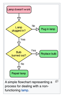
A flowchart is a type of diagram that represents a workflow or process. A flowchart can also be defined as a diagrammatic representation of an algorithm, a step-by-step approach to solving a task.
Figure 2 | Repair Flowchart for a Lamp | https://en.wikipedia.org/wiki/Flowchart |
---|---|---|
The flowchart shows the steps as boxes of various kinds, and their order by connecting the boxes with arrows. This diagrammatic representation illustrates a solution model to a given problem. Flowcharts are used in analyzing, designing, documenting or managing a process or program in various fields.
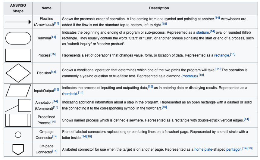
There is a symbol convention (a language) as depicted in Figure 2 below (from: https://en.wikipedia.org/wiki/Flowchart)
Figure 1 | Flowchart Symbols | https://en.wikipedia.org/wiki/Flowchart |
---|---|---|
IBM engineers implemented programming flowcharts based upon Goldstine and von Neumann's unpublished report, "Planning and coding of problems for an electronic computing instrument, Part II, Volume 1" (1947), which is reproduced in von Neumann's collected works.
The flowchart became a popular tool for describing computer algorithms, but its popularity decreased in the 1970s, when interactive computer terminals and third-generation programming languages became common tools for computer programming, since algorithms can be expressed more concisely as source code in such languages. Often pseudo-code is used, which uses the common idioms of such languages without strictly adhering to the details of a particular one.
Nowadays flowcharts are still used for describing computer algorithms.[9] Modern techniques such as UML activity diagrams and Drakon-charts can be considered to be extensions of the flowchart.
Nearly all flowcharts focus on on some kind of control, rather than on the particular flow itself! While quaint today, they are an effective way to document processes in a program and visualize structures. We recomend you get in the habit of making rudimentary flowcharts, at least at the supervisory level (the sandwich chart above)
(paraphrased from https://www.breezetree.com/articles/top-reasons-to-flowchart)
Sometimes it's more effective to visualize something graphically that it is to describe it with words. That is the essence of what flowcharts do for you. Flowcharts explain a process clearly through symbols and text. Moreover, flowcharts give you the gist of the process flow in a single glance. The following are some of the more salient reasons to use flowcharts.
Process Documentation / Training Materials Another common use for flowcharts is to create process documentation. Although this reason overlaps with regulatory and quality management requirements (below), many non-regulated businesses use flowcharts for their documentation as well. These can range in form from high-level procedures to low-level, detailed work instructions.
You may think that this applies mainly to large organizations, but small companies can greatly benefit from flowcharting their processes as well. Small enterprises need to be nimble and organized. Standardizing their processes is a great way to achieve this. In fact, the popular entrepreneurial book The E-Myth Revisited: Why Most Small Businesses Don't Work and What to Do About It by Michael Gerber is based on the fact that small businesses are more likely to succeed if they treat their operations like a franchise. in a nutshell, this means standardizing and documenting their business processes. There's no better way to do that than with flowcharts, right?
Training materials are often created using flowcharts because they're visually stimulating and easy to understand. A nicely laid out flowchart will gain and hold the reader's attention when a block of text will often fail.
Workflow Management and Continuous Improvement Workflows don't manage themselves. To ensure that you are meeting your customers' needs, you need to take control of your business processes. The first step to workflow management is to define the current state of your processes by creating an "As-Is Flowchart". That allows you to analyze your processes for waste and inefficiency. After you have identified areas for process improvement, you can then craft new flowcharts to document the leaner processes.
Programming Information technology played a big influence on the use and spread of flowcharts in the 20th century. While Dr. W. Edwards Deming was advocating their use in quality management, professionals in the data processing world were using them to flesh out their programming logic. Flowcharts were a mainstay of procedural programming, however, and with the advent of object oriented programming and various modeling tools, the use of flowcharts for programming is no longer as commonplace as it once was.
That said, even with in the scope of object oriented programming, complex program logic can be modeled effectively using a flowchart. Moreover, diagramming the user's experience as they navigate through a program is a valuable prerequisite prior to designing the user interface. So flowcharts still have their place in the world of programming.
Troubleshooting Guides Most of us have come across a troubleshooting flowchart at one time or another. These are usually in the form of Decision Trees that progressively narrow the range of possible solutions based on a series of criteria. The effectiveness of these types of flowcharts depends on how neatly the range of problems and solutions can fit into a simple True/False diagnosis model. A well done troubleshooting flowcharts can cut the problem solving time greatly.
Regulatory and Quality Management Requirements Your business processes may be subject to regulatory requirements such as Sarbanes-Oxley (SOX), which requires that your accounting procedures be clearly defined and documented. An easy way to do this is to create accounting flowcharts for all your accounting processes.
Similarly, many organizations fall under certification requirements for quality management systems - such as ISO 9000, TS 16949, or one of the many others. In such environments, flowcharts are not only useful but in certain clauses they are actually mandated.
Advanced/Optional Topic
A frequent task in data science, engineering, etc. is the seemingly mundane task of sorting or ordering things. Here we explore a couple of simple sorting algorithms, just to show some of the thoughts that go into such a task, then will ultimately resort to the internal sorting routines built into Python.
Sorting is frequently necessary when data are being handled; for example in integration and differentiation the data are usually presented to the various algorithms in ascending or descending order (at least on the x-axis). One may have tables of numbers, representing one or more explanatory variables, and one or more responses. At times we may need to arrange these tables in an order dictated by one or another of these various variables. Alternatively we may want to nd the median value or upper quartile of such a list { this task requires sorting. When sorting, one can also carry along operations to maintain correspondence with other lists (for lack of better name lets call this sort-and-carry). Tasks that fall under the broad category of sorting are:
Rank ; given an array, prepare a rank table that tells the numerical rank of an array
element.
The task of sorting N
elements requires on the order of $K \cdot Nlog2N$ operations. The
algorithm inventor tries to make $K$ as small as possible (understanding that $K = 0$ is
practically impossible). Three useful sorting algorithms are:
The choice of method depends on the size of the list that needs to be sorted. If the list is short (perhaps $N < 50$ elements) then straight insertion is fast enough, concise, and simple to program. For a long list ($N > 1000$ elements) Quicksort is faster, but achieves the speed by use of extra memory. Heapsort is also good for large lists, and is an in-place routine.
Python lists have a built-in sort()
method that modifies the list in-place and a sorted()
built-in function that builds a new sorted list from an iterable. So when sorting needs to
be done, you should use the built-in tools. However, because it is a useful programming
construct, the three sorting algorithms are presented as Python primitive codes.
The bubble sort is a place to start despite it's relative slowness. It is a pretty reviled algorithm (read the Wikipedia entry), but it is the algorithm that a naive programmer might cobble together in a hurry, and despite its shortcomings (it's really slow and inefficient), it is robust.
Here is a description of the sorting task as described by Christian and Griffths (2016) (pg. 65):
"Imagine you want to alphabetize your unsorted collection of books. A natural approach would be just to scan across the shelf looking for out- of-order pairs - Wallace followed by Pynchon, for instance - and flipping them around. Put Pynchon ahead of Wallace, then continue your scan, looping around to the beginning of the shelf each time you reach the end. When you make a complete pass without finding any more out-of-order pairs on the entire shelf, then you know the job is done. This process is a Bubble Sort, and it lands us in quadratic time. There are n books out of order, and each scan through the shelf can move each one at most one position. (We spot a tiny problem, make a tiny fix.) So in the worst case, where the shelf is perfectly backward, at least one book will need to be moved n positions. Thus a maximum of n passes through n books, which gives us O(n2) in the worst case. For instance, it means that sorting five shelves of books will take not five times as long as sorting a single shelf, but twenty-five times as long."
Converting the word description into Python is fairly simple. We will have a vector of n numbers (we use a vector because its easy to step through the different positions), and we will scan through the vector once (and essentially find the smallest thing), and put it into the first position. Then we scan again from the second position and find the smallest thing remaining, and put it into the second position, and so on until the last scan which should have the remaining largest thing. If we desire a decreasing order, simply change the sense of the comparison.
The algorithm defines an array and then sorts by repeated passes through the array. The program (outside of the sorting algorithm) is really quite simple.
#array = [7,11,5,8,9,13,66,99,223]
#array = [7,11,5]
array=[1003 ,3.2 ,55.5 , -0.0001 , -6 ,666.6 ,102]
howMany = len(array)
print("Item Count = : ",howMany)
print("Unsorted List : ", array)
# insertion sort
for irow in range(0, howMany-1) :
for jrow in range(0,(howMany-1-irow)) :
if array[jrow]> array[jrow+1] :
swap = array[jrow]
array[jrow]=array[jrow+1]
array[jrow+1]=swap
else:
continue
#results
print("Sorted List : ", array, end ="")
In the script we see that the program (near the bottom of the file) assigns the values to the vector named array and the initial order of the array is ${1003, 3.2, 55.5,-0.0001,-6, 666.6, 102}$. The smallest value in the example is -6 and it appears in the 5-th position, not the 1-st as it should.
The first pass through the array will move the largest value, 1003, in sequence to the right until it occupies the last position. Repeated passes through the array move the remaining largest values to the right until the array is ordered. One can consider the values of the array at each scan of the array as a series of transformations (irow-th scan) -- in practical cases we don't necessarily care about the intermediate values, but here because the size is manageable and we are trying to get our feet wet with algorithms, we can look at the values. The sequence of results (transformations) after each pass through the array is shown in the following list:
The next type of sorting would be to select one item and locate it either left or right of an adjacent item based on its size { like sorting a deck of cards, or perhaps a better description { again using the bookshelf analog from Christian and Griffths (2016) (pg. 65)
You might take a different tack -- pulling all the books off the shelf and putting them back in place one by one. You'd put the ffrst book in the middle of the shelf, then take the second and compare it to the first, inserting it either to the right or to the left. Picking up the third book, you'd run through the books on the shelf from left to right until you found the right spot to tuck it in. Repeating this process, gradually all of the books would end up sorted on the shelf and you'd be done. Computer scientists call this, appropriately enough, Insertion Sort. The good news is that it's arguably even more intuitive than Bubble Sort and doesn't have quite the bad reputation. The bad news is that it's not actually that much faster. You still have to do one insertion for each book. And each insertion still involves moving past about half the books on the shelf, on average, to find the correct place. Although in practice Insertion Sort does run a bit faster than Bubble Sort, again we land squarely, if you will, in quadratic time. Sorting anything more than a single bookshelf is still an unwieldy prospect." Listing 8 is an R implementation of a straight insertion sort. The script is quite compact, and I used indentation and extra line spacing to keep track of the scoping delimiters. The sort works as follows, take the an element of the array (start with 2 and work to the right) and put it into a temporary location (called swap in my script). Then compare locations to the left of swap. If smaller, then break from the loop, exchange values, otherwise the values are currently ordered. Repeat (starting at the next element) , when all elements have been traversed the resulting vector is sorted. Here are the transformations for each pass through the outer loop:
The straight insertion sort is the algorithm a card player would use to sort cards. Pick out the second card and put it into order with respect to the first; then pick the third card and insert it into sequence with the first two; continue until the last card is picked out and inserted. Once the last card is sequenced, the result is a sorted deck (list). Python implementation of such an algorithm is:
#array = [7,11,5,8,9,13,66,99,223]
array = [7,11,5]
howMany = len(array)
print("Item Count = : ",howMany)
print("Unsorted List : ", array, end ="")
# insertion sort
for i in range(1, len(array)): # Traverse through 1 to len(arr)
key = array[i]
# Move elements of arr[0..i-1], that are
# greater than key, to one position ahead
# of their current position
j = i-1
while j >=0 and key < array[j] :
array[j+1] = array[j]
j -= 1
array[j+1] = key
#results
print("Sorted List : ", array, end ="")
Probably useful to put into a functional structure:
# Function to do insertion sort
def insertionSort(array):
# Traverse through 1 to len(arr)
for i in range(1, len(array)):
key = array[i]
# Move elements of arr[0..i-1], that are
# greater than key, to one position ahead
# of their current position
j = i-1
while j >=0 and key < array[j] :
array[j+1] = array[j]
j -= 1
array[j+1] = key
return(array)
array = [7,11,5,8,9,13,66,99,223]
print("Unsorted List : ", array)
insertionSort(array)
print("Sorted List : ", array, end ="")
A practical extension of these slow sorts is called the Merge Sort. It is an incredibly useful method. One simply breaks up the items into smaller arrays, sorts those arrays - then merges the sub-arrays into larger arrays (now already sorted), and nally merges the last two arrays into the nal, single, sorted array. Here is a better description, again from Christian and Griffths (2016):
" ... information processing began in the US censuses of the nineteenth century, with the development, by Herman Hollerith and later by IBM, of physical punch-card sorting devices. In 1936, IBM began producing a line of machines called \collators" that could merge two separately ordered stacks of cards into one. As long as the two stacks were themselves sorted, the procedure of merging them into a single sorted stack was incredibly straightforward and took linear time: simply compare the two top cards to each other, move the smaller of them to the new stack you're creating, and repeat until finished.
The program that John von Neumann wrote in 1945 to demonstrate the power of the stored-program computer took the idea of collating to its beautiful and ultimate conclusion. Sorting two cards is simple: just put the smaller one on top. And given a pair of two-card stacks, both of them sorted, you can easily collate them into an ordered stack of four. Repeating this trick a few times, you'd build bigger and bigger stacks, each one of them already sorted. Soon enough, you could collate yourself a perfectly sorted full deck - with a final climactic merge, like a riffe shuffle's order- creating twin, producing the desired result. This approach is known today as Merge Sort, one of the legendary algorithms in computer science."
There are several other variants related to Merge Sort; Quicksort and Heapsort being close relatives;
# Python program for implementation of MergeSort
# https://www.geeksforgeeks.org/merge-sort/
# This code is contributed by Mayank Khanna
def mergeSort(arr):
if len(arr) >1:
mid = len(arr)//2 # Finding the mid of the array
L = arr[:mid] # Dividing the array elements
R = arr[mid:] # into 2 halves
mergeSort(L) # Sorting the first half
mergeSort(R) # Sorting the second half
i = j = k = 0
# Copy data to temp arrays L[] and R[]
while i < len(L) and j < len(R):
if L[i] < R[j]:
arr[k] = L[i]
i+= 1
else:
arr[k] = R[j]
j+= 1
k+= 1
# Checking if any element was left
while i < len(L):
arr[k] = L[i]
i+= 1
k+= 1
while j < len(R):
arr[k] = R[j]
j+= 1
k+= 1
# Code to print the list
def printList(arr):
for i in range(len(arr)):
print(arr[i], end =" ")
print()
# driver code to test the above code
#if __name__ == '__main__':
arr=[1003 ,3.2 ,55.5 , -0.0001 , -6 ,666.6 ,102]
#arr = [12, 11, 13, 5, 6, 7]
print ("Given array is", end ="\n")
printList(arr)
mergeSort(arr)
print("Sorted array is: ", end ="\n")
printList(arr)
Need narrative here
# Python program for implementation of heap Sort
# To heapify subtree rooted at index i.
# n is size of heap
def heapify(arr, n, i):
largest = i # Initialize largest as root
l = 2 * i + 1 # left = 2*i + 1
r = 2 * i + 2 # right = 2*i + 2
# See if left child of root exists and is
# greater than root
if l < n and arr[i] < arr[l]:
largest = l
# See if right child of root exists and is
# greater than root
if r < n and arr[largest] < arr[r]:
largest = r
# Change root, if needed
if largest != i:
arr[i],arr[largest] = arr[largest],arr[i] # swap
# Heapify the root.
heapify(arr, n, largest)
# The main function to sort an array of given size
def heapSort(arr):
n = len(arr)
# Build a maxheap.
# Since last parent will be at ((n//2)-1) we can start at that location.
for i in range(n // 2 - 1, -1, -1):
heapify(arr, n, i)
# One by one extract elements
for i in range(n-1, 0, -1):
arr[i], arr[0] = arr[0], arr[i] # swap
heapify(arr, i, 0)
# Driver code to test above
arr=[1003 ,3.2 ,55.5 , -0.0001 , -6 ,666.6 ,102]
#arr = [ 12, 11, 13, 5, 6, 7]
heapSort(arr)
n = len(arr)
print ("Sorted array is")
for i in range(n):
print ("%d" %arr[i]),
# This code is contributed by Mohit Kumra
Need narrative here
# Python program to sort the words in lexicographical
# order
def sortLexo(my_string):
# Split the my_string till where space is found.
words = my_string.split()
# sort() will sort the strings.
words.sort()
# Iterate i through 'words' to print the words
# in alphabetical manner.
for i in words:
print( i )
# Driver code
if __name__ == '__main__':
my_string = "hello this is example how to sort " \
"the word in alphabetical manner"
# Calling function
sortLexo(my_string)
I conclude the section on sorting with one more quoted section from Christian and Griffiths (2016) about the value for sorting - which is already relevant to a lot of data science:
"The poster child for the advantages of sorting would be an Internet search engine like Google. It seems staggering to think that Google can take the search phrase you typed in and scour the entire Internet for it in less than half a second. Well, it can't - but it doesn't need to.
If you're Google, you are almost certain that (a) your data will be searched, (b) it will be searched not just once but repeatedly, and (c) the time needed to sort is somehow less valuable" than the time needed to search. (Here, sorting is done by machines ahead of time, before the results are needed, and searching is done by users for whom time is of the essence.) All of these factors point in favor of tremendous up-front sorting, which is indeed what Google and its fellow search engines do."
Computational and Inferential Thinking Ani Adhikari and John DeNero, Computational and Inferential Thinking, The Foundations of Data Science, Creative Commons Attribution-NonCommercial-NoDerivatives 4.0 International (CC BY-NC-ND) Chapters 3-6 https://www.inferentialthinking.com/chapters/03/programming-in-python.html
Learn Python the Hard Way (Online Book) (https://learnpythonthehardway.org/book/) Recommended for beginners who want a complete course in programming with Python.
LearnPython.org (Interactive Tutorial) (https://www.learnpython.org/) Short, interactive tutorial for those who just need a quick way to pick up Python syntax.
Brian Christian and Tom Griffiths (2016) ALGORITHMS TO LIVE BY: The Computer Science of Human Decisions Henry Holt and Co. (https://www.amazon.com/Algorithms-Live-Computer-Science-Decisions/dp/1627790365)
import sys
! hostname
! whoami
print(sys.executable)
print(sys.version)
print(sys.version_info)