Download this page as a jupyter notebook at Lesson 1

ENGR 1330 Computational Thinking with Data Science

Copyright © 2021 Theodore G. Cleveland and Farhang Forghanparast

Last GitHub Commit Date: 13 July 2021

Lesson 1 Problem Solving with Computational Thinking:

• Computational thinking and problem solving
• Programming as a problem solving process
• CCMR Approach

# Script block to identify host, user, and kernel
import sys
! hostname; ! whoami; ! pwd; 
print(sys.executable)

atomickitty
sensei
/home/sensei/engr-1330-webroot/1-Lessons/Lesson01
/opt/jupyterhub/bin/python3

%%html
<!-- Script Block to set tables to left alignment -->
<style>
  table {margin-left: 0 !important;}
</style>

Computational Thinking and Problem Solving

Computational thinking (CT) refers to the thought processes involved in expressing solutions as computational steps or algorithms that can be carried out by a computer.

CT is literally a process for breaking down a problem into smaller parts, looking for patterns in the problems, identifying what kind of information is needed, developing a step-by-step solution, and implementing that solution.

1. Decomposition is the process of taking a complex problem and breaking it into more manageable sub-problems. Decomposition often leaves a framework of sub-problems that later have to be assembled (system integration) to produce a desired solution.
2. Pattern Recognition refers to finding similarities, or shared characteristics of problems, which allows a complex problem to become easier to solve, and allows use of same solution method for each occurrence of the pattern.
3. Abstraction is the process of identifying important characteristics of the problem and ignore characteristics that are not important. We use these characteristics to create a representation of what we are trying to solve.
4. Algorithms are step-by-step instructions of how to solve a problem
5. System Integration (implementation)is the assembly of the parts above into the complete (integrated) solution. Integration combines parts into a program which is the realization of an algorithm using a syntax that the computer can understand.

Programming as a problem solving process

The entire point of this course is to develop problem solving skills and begin using some tools (Statistics, Numerical Methods, Data Science, implemented as JupyterLab/Python programs).

The scientific method (https://en.wikipedia.org/wiki/Scientific_method) is one example of an effective problem solving strategy. Stated as a protocol it goes something like:

1. Observation: Formulation of a question
2. Hypothesis: A conjecture that may explain observed behavior. Falsifiable by an experiment whose outcome conflicts with predictions deduced from the hypothesis
3. Prediction: How the experiment should conclude if hypothesis is correct
4. Testing: Experimental design, and conduct of the experiment.
5. Analysis: Interpretation of experimental results

This protocol can be directly adapted to CT/DS problems as:

1. Define the problem (problem statement)
2. Gather information (identify known and unknown values, and governing equations)
3. Generate and evaluate potential solutions
4. Refine and implement a solution
5. Verify and test the solution.

For actual computational methods the protocol becomes:

1. Explicitly state the problem
2. State:
   • Input information
   • Governing equations or principles, and
   • The required output information.
3. Work a sample problem by-hand for testing the general solution.
4. Develop a general solution method (coding).
5. Test the general solution against the by-hand example, then apply to the real problem.

Oddly enough the first step is the most important and sometimes the most difficult. In a practical problem, step 2 is sometimes difficult because a skilled programmer is needed to translate the governing principles into an algorithm for the general solution (step 4).

Example 1 Problem Solving Process

Consider a need to compute an arithmetic mean, what would the process look like?

Step 1. Develop script to compute the arithmetic mean of a stream of data of unknown length.

Step 2.

• Inputs: The data stream
• Governing equation: $ \bar x = \frac{1}{N} \sum_{i=1}^{N} x_i $ where $N$ is the number of items in the data stream, and $x_i$ is the value of the i-th element.
• Outputs: The arithmetic mean $\bar x$

Step 3. Work a sample problem by-hand for testing the general solution.

Data
23.43
37.43
34.91
28.37
30.62

The arithmetic mean requires us to count how many elements are in the data stream (in this case there are 5) and compute their sum (in this case 154.76), and finally divide the sum by the count and report this result as the arithmetic mean.

$$ \bar x = \frac{1}{5}(23.43+37.43+34.91+28.37+30.62)=\frac{154.76}{5}=30.95 $$

Step 4. Develop a general solution (code)

The by-hand exercise helps identify the required steps in an “algorithm” or recipe to compute mean values. First we essentially capture or read the values then count how many there are (either as we go or as a separate step), then sum the values, then divide the values by the count, and finally report the result.

In a flow-chart it would look like:

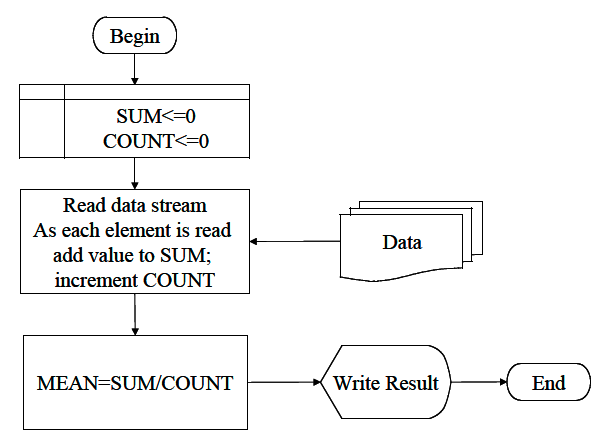
	Flowchart for Artihmetic Mean Algorithm

Step 5. This step we would code the algorithm expressed in the figure and test it with the by-hand data and other small datasets until we are convinced it works correctly.

In a simple JupyterLab script

# Arithmetic Mean in Very Elementary and Primative Python
xlist = [23.43,37.43,34.91,28.37,30.62] # list is a type of data structure
howlong = len(xlist) # len is a built-in function that returns how many items in a list
accumulator = 0 # a variable to accumulate the sum
for i in range(howlong):
    accumulator = accumulator + xlist[i]
print("arithmetic mean = ",(accumulator/howlong))

arithmetic mean =  30.951999999999998

Step 6. This step we would refine the code to generalize the algorithm. In the example we want a way to supply the xlist from a file perhaps, and tidy the output by rounding to only two decimal places - rounding is relatively simple:

# Arithmetic Mean in Very Elementary and Primative Python
xlist = [23.43,37.43,34.91,28.37,30.62] # list is a type of data structure
howlong = len(xlist) # len is a built-in function that returns how many items in a list
accumulator = 0 # a variable to accumulate the sum
for i in range(howlong):
    accumulator = accumulator + xlist[i]
print("arithmetic mean = ",round((accumulator/howlong),2))

arithmetic mean =  30.95

Reading from a file, is a bit more complicated. We need to create a connection to the file, then read the contents into our script, then put the contents into the xlist

xlist=[] # list (null) is a type of data structure
externalfile = open("data.txt",'r') # create connection to file, set to read (r), file must exist
how_many_lines = 0
for line in externalfile: # parse each line, append to xlist
    xlist.append(line)
    how_many_lines += 1
externalfile.close() # close the file connection

howlong = len(xlist) # len is a built-in function that returns how many items in a list
accumulator = 0 # a variable to accumulate the sum
for i in range(howlong):
    accumulator = accumulator + float(xlist[i])
print("arithmetic mean = ",round((accumulator/howlong),2))

arithmetic mean =  30.95

Finally, if we want to reuse the code a lot, it is convienent to make it into a function

def average(inputlist):
# inputlist should be a list of values
    howlong = len(inputlist) # len is a built-in function that returns how many items in a list
    accumulator = 0 # a variable to accumulate the sum
    for i in range(howlong):
        accumulator = accumulator + float(inputlist[i])
    result = (accumulator/howlong)
    return(result)

Put our file reading and compute mean code here

xlist=[] # list (null) is a type of data structure
externalfile = open("data.txt",'r') # create connection to file, set to read (r), file must exist
how_many_lines = 0
for line in externalfile: # parse each line, append to xlist
    xlist.append(line)
    how_many_lines += 1
externalfile.close() # close the file connection
print("arithmetic mean = ",round(average(xlist),2))

arithmetic mean =  30.95

So the simple task of computing the mean of a collection of values, is a bit more complex when decomposed that it first appears, but illustrates a five step process (with a refinement step). Throughout the course this process is always in the background.

CCMR Approach

A lot of the problems we will encounter from a CT/DS perspective have already been solved, or at least analogs have been solved. It is perfectly acceptable to use prior work for a new set of conditions as long as proper attribution is made. We call this process CCMR:

1. Copy: Find a solution to your problem from some online example: SourceForge, StackOverflow, GeeksForGeeks, DigitalOcean, etc.
2. Cite: Cite the original source. In general a citation will look like one of the references below, but a URL to the source is sufficient at first.
3. Modify: Modify the original cited work for your specific needs. Note the changes in the code using comment statements.
4. Run: Apply the modified code to the problem of interest.

In cases where we apply CCMR we are scaffolding parts (https://en.wikipedia.org/wiki/Scaffold_(programming)) - a legitimate and valuable engineering activity.

Readings

Computational and Inferential Thinking Ani Adhikari and John DeNero, Computational and Inferential Thinking, The Foundations of Data Science, Creative Commons Attribution-NonCommercial-NoDerivatives 4.0 International (CC BY-NC-ND) Chapter 1 https://www.inferentialthinking.com/chapters/01/what-is-data-science.html

Learn Python the Hard Way (Online Book) (https://learnpythonthehardway.org/book/) Recommended for beginners who want a complete course in programming with Python.

LearnPython.org (Interactive Tutorial) (https://www.learnpython.org/) Short, interactive tutorial for those who just need a quick way to pick up Python syntax.

How to Think Like a Computer Scientist (Interactive Book) (https://runestone.academy/runestone/books/published/thinkcspy/index.html) Interactive "CS 101" course taught in Python that really focuses on the art of problem solving.

How to Learn Python for Data Science, The Self-Starter Way (https://elitedatascience.com/learn-python-for-data-science)

Theodore G. Cleveland, Farhang Forghanparast, Dinesh Sundaravadivelu Devarajan, Turgut Batuhan Baturalp (Batu), Tanja Karp, Long Nguyen, and Mona Rizvi. (2021) Computational Thinking and Data Science: A WebBook to Accompany ENGR 1330 at TTU, Whitacre College of Engineering, DOI (pending)http://54.243.252.9/engr-1330-webroot/engr-1330-webbook/ctds-psuedocourse/site/