Numerical Methods -- Integration
At this point we have enough Python to consider doing some useful computations. We will start with numerical integration because it is useful and only requires count-controlled repetition and single subscript lists.
Background
Numerical integration is the numerical approximation of
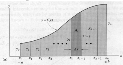
\begin{equation} I = \int_a^b f(x)dx \end{equation}Consider the problem of determining the shaded area under the curve $y = f(x)$ from $x = a$ to $x = b$, as depicted in the figure below, and suppose that analytical integration is not feasible.

Aside: How to embed a figure
1) Upload the file to the notebook directory, for this kind of environment use .png, .jpg
2) Use the markdown syntax . I used ""
3) The [] is a tag delimiter, I dont know how to use tags yet, its not a caption (bummer!)
The function may be known in tabular form from experimental measurements or it may be known in an analytical form. The function is taken to be continuous within the interval $a < x < b$. We may divide the area into $n$ vertical panels, each of width $\Delta x = (b - a)/n$, and then add the areas of all strips to obtain $A~\approx \int ydx$.
A representative panel of area $A_i$ is shown with darker shading in the figure. Three useful numerical approximations are listed in the following sections. The approximations differ in how the function is represented by the panels --- in all cases the function is approximated by known polynomial models between the panel end points.
In each case the greater the number of strips, and correspondingly smaller value of $\Delta x$, the more accurate the approximation. Typically, one can begin with a relatively small number of panels and increase the number until the resulting area approximation stops changing.
Rectangular Panels -- in primatives
A primative is a structure built with the base python language and avoids packages, in my work it is obvious, the import package.name is absent in the source code.
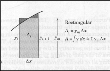
The figure below is a schematic of a rectangular panels. The figure is assuming the function structure is known and can be evaluated at an arbitrary location in the $\Delta x$ dimension.

Each panel is treated as a rectangle, as shown by the representative panel whose height $y_m$ is chosen visually so that the small cross-hatched areas are as nearly equal as possible. Thus, we form the sum $\sum y_m$ of the effective heights and multiply by $\Delta x$. For a function known in analytical form, a value for $y_m$ equal to that of the function at the midpoint $x_i + \Delta x /2$ may be calculated and used in the summation.
For tabulated functions, we have to choose to either take $y_m$ as the value at the left endpoint or right endpoint. This limitation is often quite handy when we are trying to integrate a function that is integrable, but undefined on one endpoint.
Lets try some examples in Python.
Find the area under the curve $y= x\sqrt{1+x^2}$ from $x = 0$ to $x = 2$.
First lets read in the value for the lowerlimit, we will do some limited error checks to be sure user enters a number, but won't check that the number is non-negative.
# RectangularPanels.py
# Numerical Integration
print ("Program finds area under curve y = x * sqrt(1+x)")
# Get input data -- use error checking
yes = 0
while yes == 0:
    x_low = input("Enter a lower bound x_low \n")
    try:
        x_low = float(x_low)
        yes = 1
    except:
        print ("x_low really needs to be a number, try again \n")
# exit the while loop when finally have a valid number
Verify that value is indeed what we entered
print(x_low)
Now do the same for the upper limit, notice how we are using the yes variable. We set a "fail" value, and demand input until we get "success". The structure used here is called a try -- exception structure and is very common in programming. Error checking is really important so that garbled input does not hang things up.
yes = 0
while yes == 0:
    x_high = input("Enter an upper bound x_high \n")
    try:
        x_high = float(x_high)
        yes = 1
    except:
        print ("x_high really needs to be a number, try again \n")
# exit the while loop when finally have a valid number
Again verify!
print(x_high)
Now use the try - exception structure to input how many panels we wish to use. Notice you can enter a negative value which will ultimately break things. Also observe this value is an integer.
yes = 0
while yes == 0:
    how_many = input("Enter how many panels \n")
    try:
        how_many = int(how_many)
        yes = 1
    except:
        print ("Panels really needs to be a number, try again \n")
# exit the while loop when finally have a valid number
Again verify!
print(how_many)
Now we can actually perform the integration by evaluating the function at the panel half-widths.
In this example we are using primitive arithmetic, so the $\sqrt{}$ is accomplished by exponentation, the syntax is c = a ** b is the operation $c = a^b$.
The integration uses an accumulator, which is a memory location where subsquent results are added (accumulated) back into the accumulator. This structure is so common that there are alternate, compact syntax to perform this task, here it is all out in the open.
The counting loop where we evaluate the function at different x values, starts at 1 and ends at how_many+1 because python for loops use an increment skip if equal structure. When the value in range equals how_many the for loop exits (break is implied.) A loop control structure starting from 0 is shown in the code as a comment line. Simply uncomment this line, and comment the line just below to have the structure typical in python scripts. In the start from 1 case, we want to evaluate at the last value of how_many.
# OK we should have the three things we need for evaluating the integral
delta_x = (x_high - x_low)/float(how_many)  # compute panel width
xx = x_low + delta_x/2 # initial value for x
### OK THIS IS THE ACTUAL INTEGRATOR PART ###
accumulated_area = 0.0  # initial value in an accumulator
#for i in range(0,how_many,1): #note we are counting from 0
for i in range(1,how_many+1,1): #note we are counting from 1
    accumulated_area = accumulated_area + ( xx * ( (1+xx**2)**(0.5) ) ) * delta_x
    xx = xx + delta_x
### AND WE ARE DONE INTEGRATING #############
Finally, we want to report our result
print ("Area under curve y = x * sqrt(1+x) from x = ",x_low,\
      " to x = ",x_high,"\n is approximately: ",accumulated_area)
# the backslash \
#       " to x = .....     lets us use multiple lines
# the \n is a "newline" character
The code implements rudimentary error checking -- it forces us to enter numeric values for the lower and upper values of $x$ as well as the number of panels to use. It does not check for undefined ranges and such, but you should get the idea -- notice that a large fraction of the entire program is error trapping; this devotion to error trapping is typical for professional programs where you are going to distribute executable modules and not expect the end user to be a programmer.
Using the math package
The actual computations are done rather crudely -- there is a math package that would give us the ability to compute the square root as a function call rather than exponentiation to a real values exponent.
That is illustrated below
# RectangularPanels.py
# Numerical Integration
# Use built-in math functions
import math  # a package of math functions
# we are naming an object "sqrt" that will compute the square root
def sqrt (x):
        return math.sqrt(x)
# saves us having to type math.NAME every time we wish to use a function
# in this program not all that meaningful, but in complex programs handy!
print ("Program finds area under curve y = x * sqrt(1+x)")
# Get input data -- use error checking
yes = 0
while yes == 0:
    x_low = input("Enter a lower bound x_low \n")
    try:
        x_low = float(x_low)
        yes = 1
    except:
        print ("x_low really needs to be a number, try again \n")
yes = 0
while yes == 0:
    x_high = input("Enter an upper bound x_high \n")
    try:
        x_high = float(x_high)
        yes = 1
    except:
        print ("x_high really needs to be a number, try again \n")
yes = 0
while yes == 0:
    how_many = input("Enter how many panels \n")
    try:
        how_many = int(how_many)
        yes = 1
    except:
        print ("Panels really needs to be a number, try again \n")
delta_x = (x_high - x_low)/float(how_many)  # compute panel width
accumulated_area = 0.0  # initial value in an accumulator
xx = x_low + delta_x/2 # initial value for x
for i in range(1,how_many+1,1): #note we are counting from 1
    accumulated_area = accumulated_area + ( xx * sqrt(1+xx**2) ) * delta_x
    xx = xx + delta_x
print ("Area under curve y = x * sqrt(1+x) from x = ",x_low,\
      " to x = ",x_high,"\n is approximately: ",accumulated_area)
Trapezoidal Panels
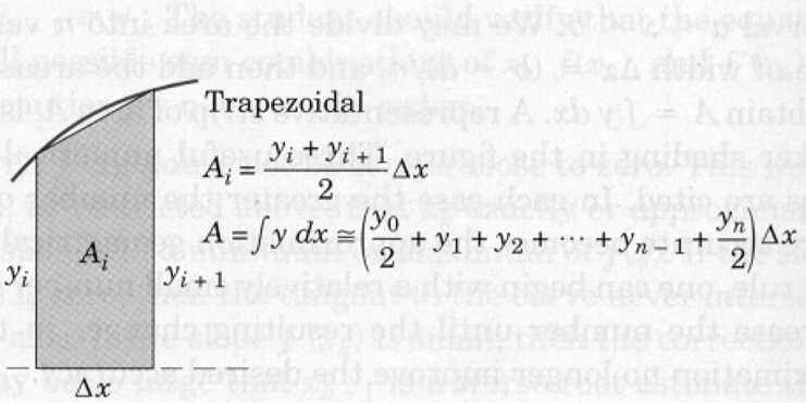
The trapezoidal panels are approximated as shown in the figure below.

The area $A_i$ is the average height $(y_i + y_{i+1} )/2$ times $\Delta x$. Adding the areas gives the area approximation as tabulated. For the example with the curvature shown, the approximation will be on the low side. For the reverse curvature, the approximation will be on the high side. The trapezoidal approximation is commonly used with tabulated values.
The script below illustrates the trapezoidal method for approximating an integral. In the example, the left and right panel endpoints in $x$ are set as separate variables $x_{left}$ and $x_{right}$ and incremented by $\Delta x$ as we step through the count-controlled repetition to accumulate the area. The corresponding $y$ values are computed within the loop and averaged, then multiplied by $\Delta x$ and added to the accumulator. Finally the $x$ values are incremented --- for grins, we used the += operator on the accumulator
# TrapezoidalPanels.py
# Numerical Integration
# Use built-in math functions
import math  # a package of math functions
# we are naming an object "sqrt" that will compute the square root
def sqrt (x):
        return math.sqrt(x)
# saves us having to type math.NAME every time we wish to use a function
# in this program not all that meaningful, but in complex programs handy!
print ("Program finds area under curve y = x * sqrt(1+x)")
# Get input data -- use error checking
yes = 0
while yes == 0:
    x_low = input("Enter a lower bound x_low \n")
    try:
        x_low = float(x_low)
        yes = 1
    except:
        print ("x_low really needs to be a number, try again \n")
yes = 0
while yes == 0:
    x_high = input("Enter an upper bound x_high \n")
    try:
        x_high = float(x_high)
        yes = 1
    except:
        print ("x_high really needs to be a number, try again \n")
yes = 0
while yes == 0:
    how_many = input("Enter how many panels \n")
    try:
        how_many = int(how_many)
        yes = 1
    except:
        print ("Panels really needs to be a number, try again \n")
delta_x = (x_high - x_low)/float(how_many)  # compute panel width
accumulated_area = 0.0      # initial value in an accumulator
x_left = x_low              # initial value for x_left edge panel
x_right = x_left + delta_x  # initial value for x_right edge panel
for i in range(1,how_many+1,1): #note we are counting from 1
    y_left = ( x_left* sqrt(1+x_left**2) )
    y_right = ( x_right* sqrt(1+x_right**2) )
    accumulated_area += + (1./2.) * ( y_left + y_right ) * delta_x
    x_left += delta_x
    x_right += delta_x
print ("Area under curve y = x * sqrt(1+x) from x = ",x_low,\
      " to x = ",x_high,"\n is approximately: ",accumulated_area)
Parabolic Panels
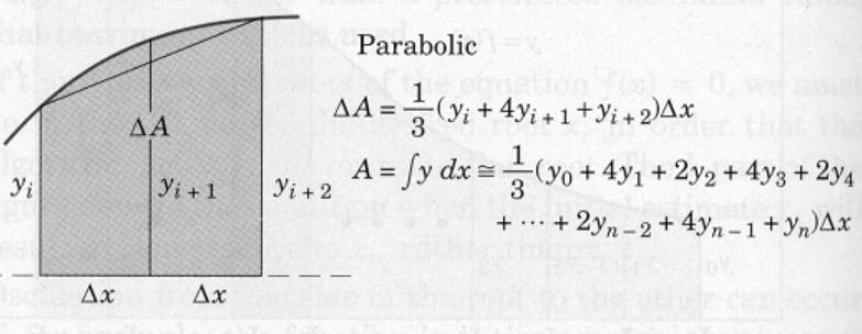
Parabolic panels approximate the shape of the panel with a parabola. The area between the chord and the curve (neglected in the trapezoidal solution) may be accounted for by approximating the function with a parabola passing through the points defined by three successive values of $y$.

This area may be calculated from the geometry of the parabola and added to the trapezoidal area of the pair of strips to give the area $\Delta A$ of the pair as illustrated. Adding all of the $\Delta A$s produces the tabulation shown, which is known as Simpson's rule. To use Simpson's rule, the number $n$ of strips must be even.
The same example as presented for rectangular panels is repeated, except using parabolic panels. The code is changed yet again because we will evaluate at each end of the panel as well as at an intermediate value.
# ParabolicPanels.py
# Numerical Integration
# Use built-in math functions
import math  # a package of math functions
# we are naming an object "sqrt" that will compute the square root
def sqrt (x):
        return math.sqrt(x)
# saves us having to type math.NAME every time we wish to use a function
# in this program not all that meaningful, but in complex programs handy!
print ("Program finds area under curve y = x * sqrt(1+x)")
# Get input data -- use error checking
yes = 0
while yes == 0:
    x_low = input("Enter a lower bound x_low \n")
    try:
        x_low = float(x_low)
        yes = 1
    except:
        print ("x_low really needs to be a number, try again \n")
yes = 0
while yes == 0:
    x_high = input("Enter an upper bound x_high \n")
    try:
        x_high = float(x_high)
        yes = 1
    except:
        print ("x_high really needs to be a number, try again \n")
yes = 0
while yes == 0:
    how_many = input("Enter how many panels \n")
    try:
        how_many = int(how_many)
        yes = 1
    except:
        print ("Panels really needs to be a number, try again \n")
delta_x = (x_high - x_low)/float(how_many)  # compute panel width
accumulated_area = 0.0         # initial value in an accumulator
x_left   = x_low               # initial value for x_left edge panel
x_middle = x_left   + delta_x  # initial value for x_middle edge panel
x_right  = x_middle + delta_x  # initial value for x_right edge panel
how_many = int(how_many/2)     # using 2 panels every step, so 1/2 many steps -- force integer result
for i in range(1,how_many+1,1): #note we are counting from 1
    y_left   = ( x_left   * sqrt(1+   x_left**2) )
    y_middle = ( x_middle * sqrt(1+ x_middle**2) )
    y_right  = ( x_right  * sqrt(1+  x_right**2) )
    accumulated_area = accumulated_area + \
                       (1./3.) * ( y_left + 4.* y_middle + y_right ) * delta_x
    x_left   = x_left   + 2*delta_x
    x_middle = x_left   +   delta_x
    x_right  = x_middle +   delta_x
print ("Area under curve y = x * sqrt(1+x) from x = ",x_low,\
      " to x = ",x_high,"\n is approximately: ",accumulated_area)
If we study all the forms of the numerical method we observe that the numerical integration method is really the sum of function values at specific locations in the interval of interest, with each value multiplied by a specific weight.
In this development the weights were based on polynomials, but other method use different weighting functions. An extremely important method is called gaussian quadrature. This method is valuable because one can approximate convolution integrals quite effectively using quadrature routines, while the number of function evaluations for a polynomial based approximation could be hopeless.
When the function values are tabular, we are going to have to accept the rectangular (with adaptations) and trapezoidal as our best tools to approximate an integral because we don't have any really effective way to evaluate the function between the tabulated values.