%%html
<!--Script block to left align Markdown Tables-->
<style>
  table {margin-left: 0 !important;}
</style>
# Preamble script block to identify host, user, and kernel
import sys
! hostname
! whoami
print(sys.executable)
print(sys.version)
print(sys.version_info)
Lesson 24 - Classification (Continued)
Lesson 23 http://54.243.252.9/engr-1330-psuedo-course/CECE-1330-PsuedoCourse/1-Lessons/Lesson23/PsuedoLesson/Lesson23-DEV.html introduced classification, and left us with an example of binary classification. The next concept is the neuron analog.
The Neuron
Animal brains puzzled scientists, because even small ones like a pigeon brain were vastly more capable than digital computers with huge numbers of electronic computing elements, huge storage space, and all running at frequencies much faster than fleshy squishy natural brains.
One explaination is architectural differences. Computers processed data sequentially, and exactly. There is no ambiguity about calculations. Animal brains, on the other hand, although apparently running at much slower rhythms, seemed to process signals in parallel, and ambiguity is a feature of their computation. The basic unit of a biological brain is the neuron:
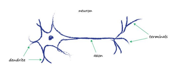
Neurons, although there are various forms of them, all transmit an electrical signal from one end to the other, from the dendrites along the axons to the terminals. These signals are then passed from one neuron to another. This is how your body senses light, sound, touch pressure, heat and so on. Signals from specialised sensory neurons are transmitted along your nervous system to your brain, which itself is mostly made of neurons too. But the neuron also functions as a logic gate - the incoming inputs have to trigger a transmission event.
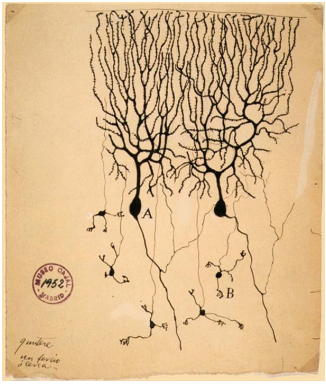
The following is a sketch of neurons in a pigeon’s brain, made by a Spanish neuroscientist in 1889. You can see the key parts - the dendrites and the terminals.
How many neurons do we need to perform interesting, more complex, tasks? Well, the very capable human brain has about 100 billion neurons! A fruit fly has about 100,000 neurons and is capable of flying, feeding, evading danger, finding food, and many more fairly complex tasks. This number, 100,000 neurons, is well within the realm of modern computers to try to replicate. A nematode worm has just 302 neurons, which is positively miniscule compared to today’s digital computer resources! But that worm is able to do some fairly useful tasks that traditional computer programs of much larger size would struggle to do. So what’s the secret? Why are biological brains so capable given that they are much slower and consist of relatively few computing elements when compared to modern computers? The complete functioning of brains, consciousness for example, is still a mystery, but enough is known about neurons to suggest different ways of doing computation, that is, different ways to solve problems. So let’s look at how a neuron works. It takes an electric input, and pops out another electrical signal. This looks exactly like the classifying or predicting machines we looked at earlier, which took an input, did some processing, and popped out an output.
Threshold triggering
So we could represent neurons as linear functions, but a biological neuron doesn’t produce an output that is simply a simple linear function of the input. That is, its output does not take the form output = (constant * input) + (maybe another constant).
Observations suggest that neurons don’t react readily, but instead suppress the input until it has grown so large that it triggers an output. You can think of this as a threshold that must be reached before any output is produced. It’s like water in a cup - the water doesn’t spill over until it has first filled the cup. Intuitively this makes sense - the neurons don’t want to be passing on tiny noise signals, only emphatically strong intentional signals. The following illustrates this idea of only producing an output signal if the input is sufficiently dialed up to pass a threshold.
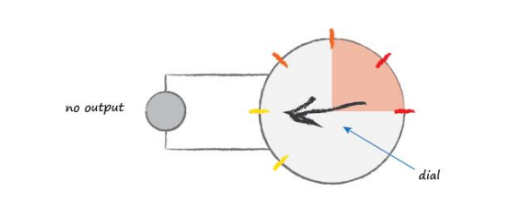
The input signal moves the dial - it is detected, but not sufficiently to trigger a change of state of the output
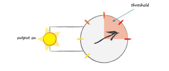
In this figure the input signal moves the dial into the threshold region and does trigger a change of state of the output
A function that takes the input signal and generates an output signal, but takes into account some kind of threshold is called an activation function. Mathematically, there are many such activation functions that could achieve this effect.
Activation Functions
A step function could serve as an activation function
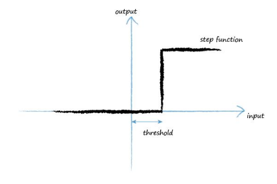
You can see for low input values, the output is zero. However once the threshold input is reached, output jumps up. An artificial neuron behaving like this would be like a real biological neuron. The term used by scientists actually describes this well, they say that neurons fire when the input reaches the threshold.
We can improve on the step function. The S-shaped function shown is called the sigmoid function (kind of looks like logistic regression eh?). It is smoother than the step function, and this makes it more natural and eliminates the discontinunity at the step.
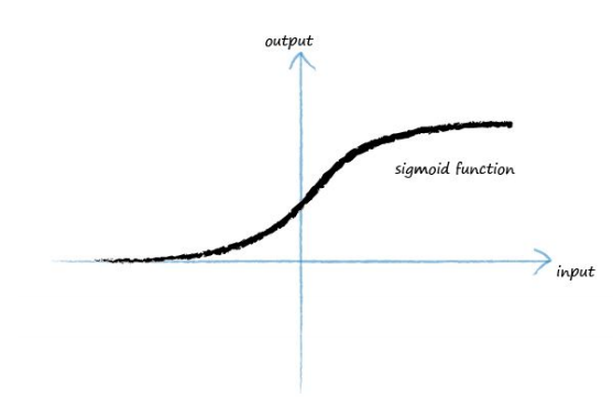
The sigmoid function, also called the logistic function, is
$$ y = \frac{1}{1+e^{-x}} $$A reason for choosing this sigmoid function over the many many other S-shaped functions we could have used for a neuron’s output is that sigmoid function is much easier to do calculations with than other S-shaped functions.
Consider how to model an artificial neuron. The first thing to realise is that real biological neurons take many inputs, not just one.
We saw this when we had multiple inputs to the linear regression, so the idea of having more than one input is not new or unusual. In a neuron we combine them by adding them up, and the resultant sum is used as the input to the sigmoid function which controls the output. This abstraction reflects how real neurons work. The following diagram illustrates this idea of combining inputs and then applying the threshold to the combined sum:
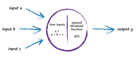
If the combined signal is not large enough then the effect of the sigmoid threshold function is to suppress the output signal. If the sum x is large enough the effect of the sigmoid is to fire the neuron. Interestingly, if only one of the several inputs is large and the rest small, this may be enough to fire the neuron. What’s more, the neuron can fire if some of the inputs are individually almost, but not quite, large enough because when combined the signal is large enough to overcome the threshold. In an intuitive way, this gives you a sense of the fuzzy calculations that such neurons can do.
The electrical signals are collected by the dendrites and these combine to form a stronger electrical signal. If the signal is strong enough to pass the threshold, the neuron fires a signal down the axon towards the terminals to pass onto the next neuron’s dendrites. The following diagram shows several neurons connected in this way:
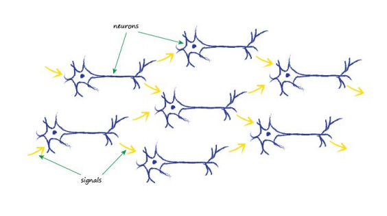
The thing to notice is that each neuron takes input from many before it, and also provides signals to many more, if it happens to be firing. One way to replicate this from nature to an artificial model is to have layers of neurons, with each connected to every other one in the preceding and subsequent layer. The following diagram illustrates this idea:
Rashid, Tariq. Make Your Own Neural Network (Page 47). . Kindle Edition.
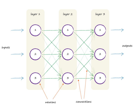
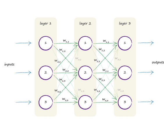
You can see the three layers, each with three artificial neurons, or nodes. You can also see each node connected to every other node in the preceding and next layers. That’s great! But what part of this cool looking architecture does the learning? What do we adjust in response to training examples? Is there a parameter that we can refine like the slope of the linear classifiers we looked at earlier? The most obvious thing is to adjust the strength of the connections between nodes. Within a node, we could have adjusted the summation of the inputs, or we could have adjusted the shape of the sigmoid threshold function, but that’s more complicated than simply adjusting the strength of the connections between the nodes. The following diagram again shows the connected nodes, but this time a weight is shown associated with each connection. A low weight will de-emphasise a signal, and a high weight will amplify it.
Signal Trace
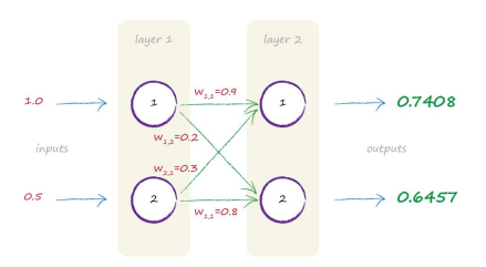
Lets manually trace a signal through a smaller neural network with only 2 layers, each with 2 neurons, as shown below:
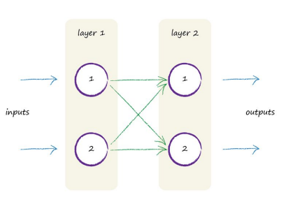
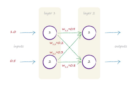
Let’s imagine the two inputs are 1.0 and 0.5, and as before, each node turns the sum of the inputs into an output using an activation function. We’ll also use the sigmoid function $y = \frac{1}{1 + e^{−x}}$ that we saw before, where x is the sum of incoming signals to a neuron, and y is the output of that neuron.
What about the weights? Let’s go with some arbitrary weights:
$w_{1,1} = 0.9$
$w_{1,2} = 0.2$
$w_{2,1} = 0.3$
$w_{2,2} = 0.8$
Random starting values aren’t such a bad idea, and it is what we did when we chose an initial slope value for the simple linear classifiers earlier on. The initial value got improved with each example that the classifier learned from. The same should be true for neural networks link weights. There are only four weights in this small neural network, as that’s all the combinations for connecting the 2 nodes in each layer. The following diagram shows all these numbers now marked.
The first layer of nodes is the input layer, and it doesn’t do anything other than represent the input signals. That is, the input nodes don’t apply an activation function to the input. The first layer of neural networks is the input layer and all that layer does is represent the inputs - that’s it.
The first input layer (Layer 1) is easy - no calculations to be done there. Next is the second layer where we do need to do some calculations. For each node in this layer we need to work out the combined input. Remember that sigmoid function, $y = \frac{1}{1 + e^{−x}}$? Well the x in that function is the combined input into a node.
That combination was the raw outputs from the connected nodes in the previous layer, but moderated by the link weights. The following diagram is like the one we saw previously but now includes the need to moderate the incoming signals with the link weights.

# script to illustrate node activation
import math
def node_trigger(input1,input2):
    inputsum = input1+input2
    response = 1.0/(1.0+math.exp(-inputsum))
    return(response)
# simple 2X2 ANN
#current weights
w11=0.9
w12=0.2
w21=0.3
w22=0.8
#inputs
in1 = 1.0
in2 = 0.5
# process layer
print('node 2-1 output',node_trigger(w11*in1,w21*in2))
print('node 2-2 output',node_trigger(w12*in1,w22*in2))
Here is a graphic of what the script does
Matrix Arithmetic
Its not too hard to imagine that it would be horrible to manually write the script for a whole bunch of nodes and many layers. However the structure is amenable to matrix representation.
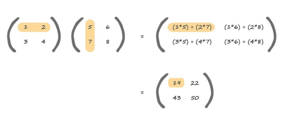
Matrix multiplication is important in classification; have a look at the following which highlights how the top left element of the answer is worked out.
# matrix vector multiply script from Lesson 19
def mvmult(amatrix,bvector,rowNumA,colNumA):
    result_v = [0 for i in range(rowNumA)]
    for i in range(0,rowNumA):
        for j in range(0,colNumA):
                result_v[i]=result_v[i]+amatrix[i][j]*bvector[j]
    return(result_v)

def sigmoid(inputsum):
    response = 1.0/(1.0+math.exp(-inputsum))
    return(response)

weights = [[0.9,0.2],[0.3,0.8]]
inputs = [1.0,0.5]
middle = mvmult(weights,inputs,2,2)

print('node 2-1 output',sigmoid(middle[0]))
print('node 2-2 output',sigmoid(middle[1]))
Multiple Classifiers (future revisions)
Neuron Analog (future revisions)
- threshold
- step-function
- logistic function
- computational linear algebra
Classifiers in Python (future revisions)
- KNN Nearest Neighbor (use concrete database as example, solids as homework)
- ANN Artifical Neural Network (use minst database as example, something from tensorflow as homework)
- Clustering(K means, heriarchial (random forests))
- SVM
- PCA (? how is this machine learning we did this in the 1970s?)
References
Rashid, Tariq. Make Your Own Neural Network. . Kindle Edition.