Download (right-click, save target as ...) this page as a Jupyterlab notebook from: ES-1
CE 5319 Machine Learning for Civil Engineers
Fall 2022 Exercise Set 1
LAST NAME, FIRST NAME
R00000000
Purpose :
Demonstrate ability to build simple (naive) prediction and classification engines using primative python.
Assessment Criteria :
Completion, results plausible, format correct, calculations (Jupyter Notebook) are shown.
Problem 1
Build a simple prediction engine for a dive computer device

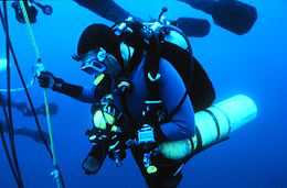
| Diver with Computer |
|---|
Background
Scuba divers circa 1980's used to memorize dive tables which provided safe depth-duration combinations (e.g. 60 feet for 60 minutes). Commerical divers used similar tables. A bounce would occur when a diver at depth notices a shiny object and descends deeper for a very short interval to recover the object - usually something worthless, but occassionally something very valuable. Bounce dives can be quite dangerous - more so if the diver is trying to adapt a memorized dive table to his/her current situation, hence the development of dive computers.
The US Navy started development of dive computers in the 1950's to relieve the human of the somewhat tricky task of multi-level dive planning and monitoring. The first digital dive computer was a laboratory model, the XDC-1, based on a desktop electronic calculator, converted to run a DCIEM four-tissue algorithm in 1975. It used pneumofathometer depth input from surface-air supplied divers.
In 1976 the diving equipment company Dacor developed and marketed a digital dive computer which used a table lookup based on stored US Navy tables rather than a real-time tissue gas saturation model. The Dacor Dive Computer (DDC), displayed output on light-emitting diodes for: current depth; elapsed dive time; surface interval; maximum depth of the dive; repetitive dive data; ascent rate, with a warning for exceeding 20 metres per minute; warning when no-decompression limit is reached; battery low warning light; and required decompression.
In the subsequent decade several firms developed and marketed dive computers; by 1989, the advent of dive computers had not met with what might be considered widespread acceptance. Combined with the general mistrust, at the time, of taking a piece of electronics that your life might depend upon underwater, there were also objections expressed ranging from dive resorts believing that the increased bottom time would upset their boat and meal schedules, to that of experienced divers who felt that the increased bottom time would, regardless of the claims, result in many more cases of decompression sickness.
By 2015 sophisticated dive computers using real-time tissue gas saturation models were commonplace and comparatively inexpensive (circa 2020 computers are programmable for exotic gasses - greatly relieving the diver's workload in planning and monitoring multi-level (bounce) dives).

| Helium-Oxygen Dive Computer Readout |
|---|
Problem Statement
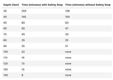
Using the data below develop a prediction for a dive computer that uses Dacor's original approach (i.e. table lookup in this case replaced by an data model). The table lists allowable time at prescribed depths for a recreational diver with a safety decompression stop at 10 feet depth.

In the context of ML the supplied table is the "truth table" and initially our goal is to fit some kind of hypothesis to this table. Avoid the temptation to just apply linear regression and instead mimic the naive learner in the class notes.
Consider the two hypothesis structures below and decide which produces a more useful model.
- $\text{Time} = \beta_{0}+\beta_{1}*\text{Depth}$
- $\text{Time} = \beta_{0}+\beta_{1}*log_{10}(\text{Depth}+\beta_{3})$
Summarize your efforts into a brief blog-post type of report (i.e. in a Jupyter Notebook)
Problem 2
Build a simple classifier to determine a bug type based upon 1200 examples supplied in the file bugs-train.csv.
Suggested Workflow:
- Download the training file.
- Perform visual EDA by plotting the two feature variables on a scatterplot, assign the class variables two colors.
- Decide if the two groups are seperable based on the EDA plot.
- Mimicing the course notes construct a classifier that automatically finds a separation line in the feature space.
- Test your classifier using bugs-test.csv.
- Then challenge the classifier with the small challenge set bugs-challenge.csv that does not contain the labels.
- Summarize your efforts into a brief blog-post type of report (i.e. in a Jupyter Notebook)