CE 4363/5363 Groundwater Hydrology
Spring 2023 Exam 2
LAST NAME, FIRST NAME
R00000000
Purpose :
Demonstrate ability to apply groundwater hydrology principles to aquifers
Additional Instructions
- The test is intended to be completed by extracting the problem statements and inserting worked answers, including computations into a document, saving that document as a PDF file, and uploading the completed exam to Blackboard.
- Show your work; handwritten is OK, but must be neat, organized, and legible (no brain vomit)
- Cite reference sources used to support your work
CE 4363 Complete problems 1-4
CE 5363 Complete problems 1-6
Problem 7 is extra credit for either course
Question 2 (30 pts.)
A confined aquifer system is conceptualized as pictured below.
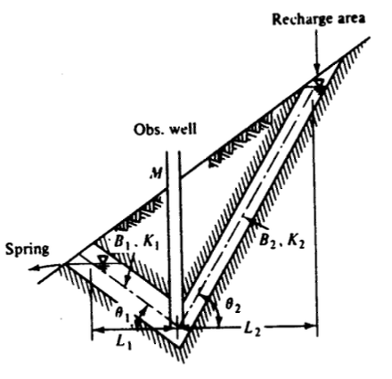
Water enters the system in the recharge area and exits as a spring.
Determine:
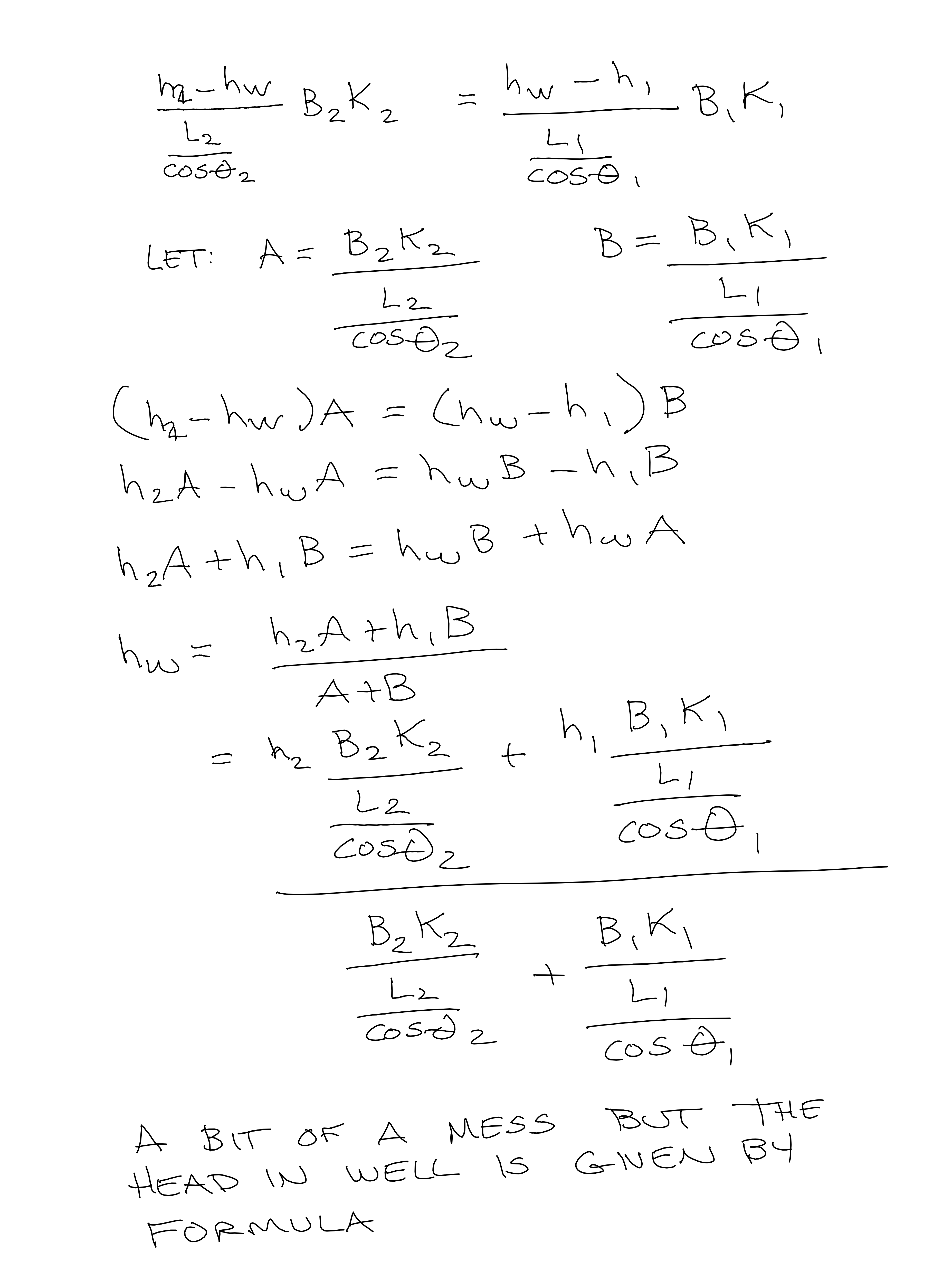
- The piezometric head in the well located at $M$ (express the head in terms of the other variables indicated on the sketch)
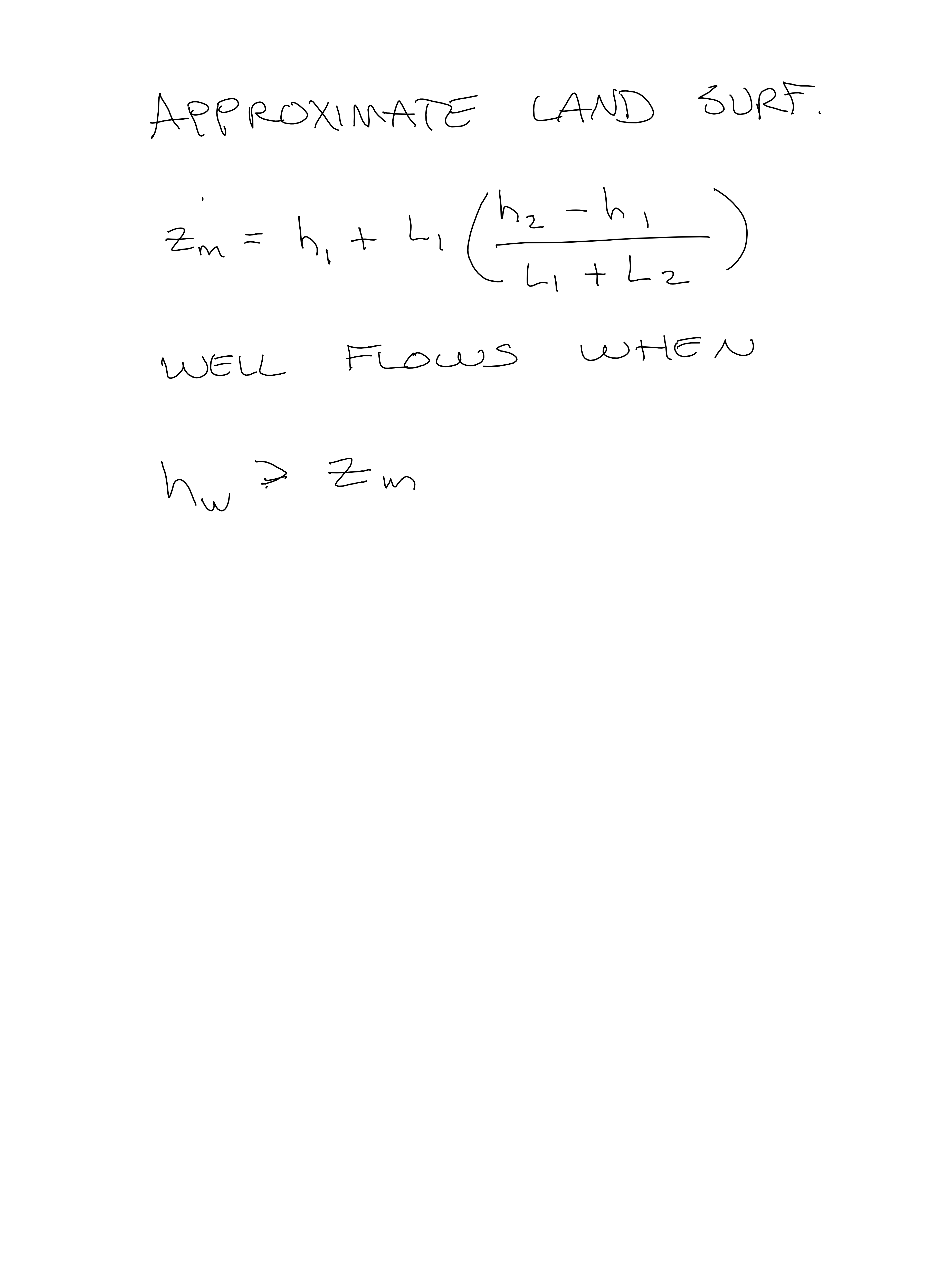
- Specify the conditions for the well to become a flowing (artesian) well (water flows from the well without pumping).

Question 3 (30 pts.)
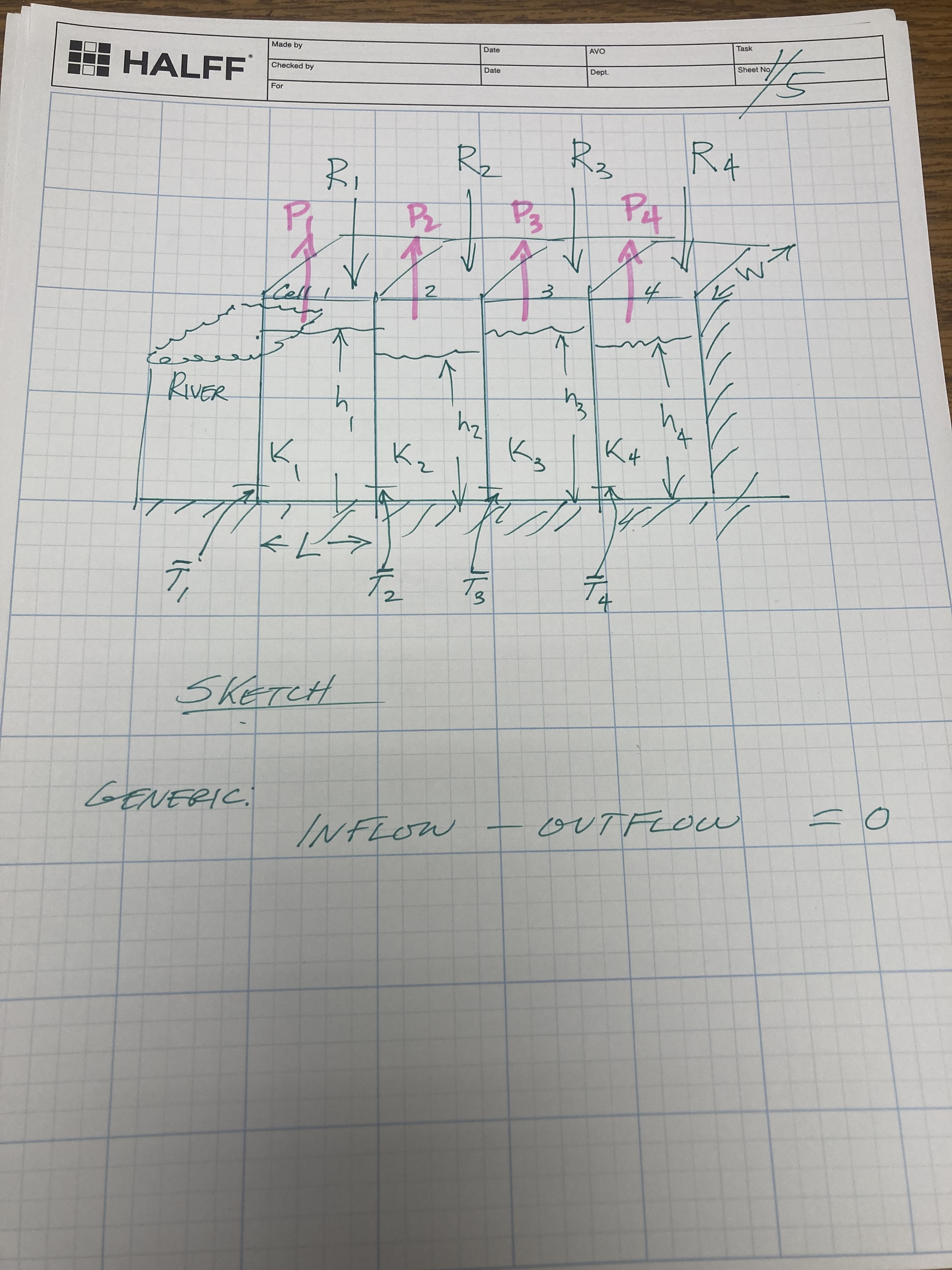
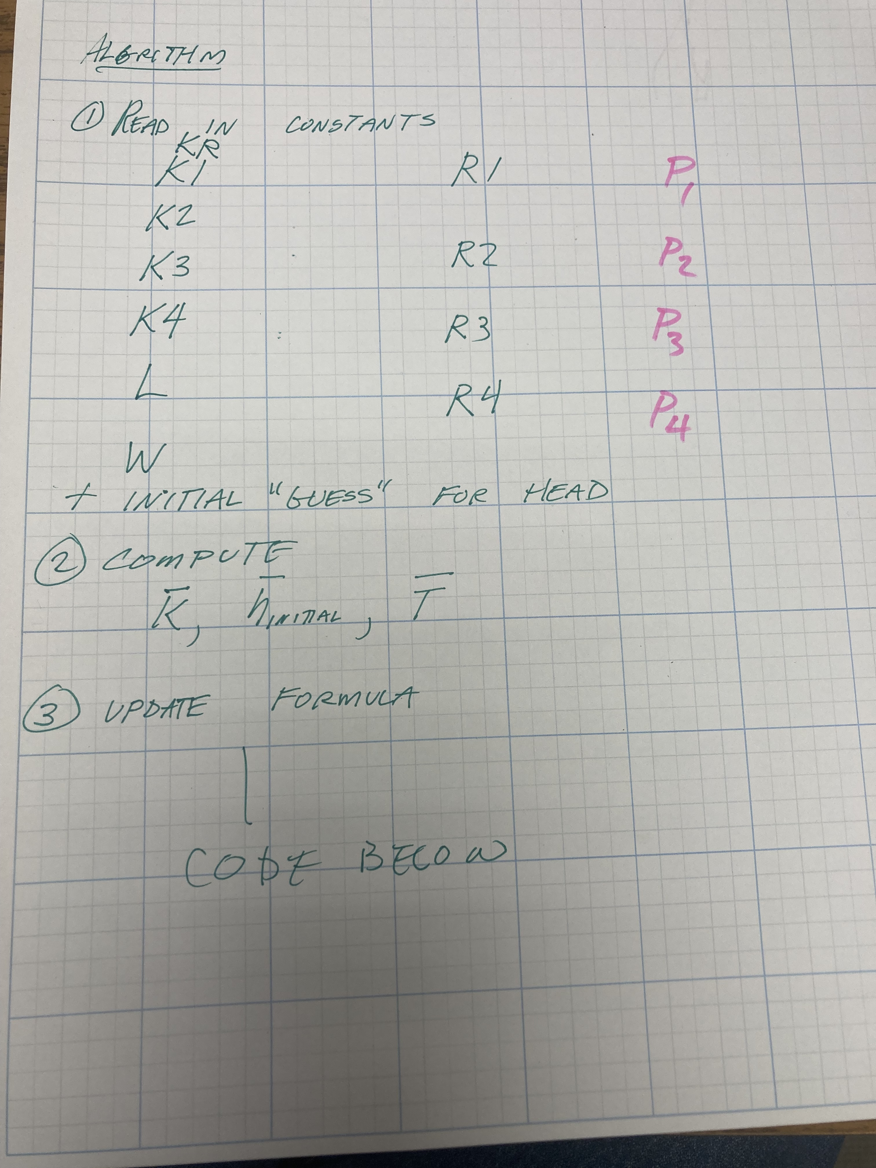
A 4-cell aquifer model is conceptualized in the figure below.
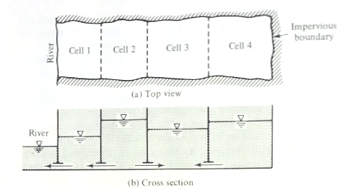
The width of the aquifer strip is 3.0 km; the length of each cell is 5 km. The recharge rates for the aquifer strip is $400~\frac{mm}{yr}$, $300~\frac{mm}{yr}$,$300~\frac{mm}{yr}$, $200~\frac{mm}{yr}$ in Cells 1,2,3, and 4, respectively. The water level in the river is maintained at a constant elevation of $160~m$ above the horizontal impervious bottom. The hydraulic conductivity in Cells 1 and 2 is $3~\frac{m}{d}$, while in Cells 3 and 4 it is $6~\frac{m}{d}$.
Using this conceptual model, determine:
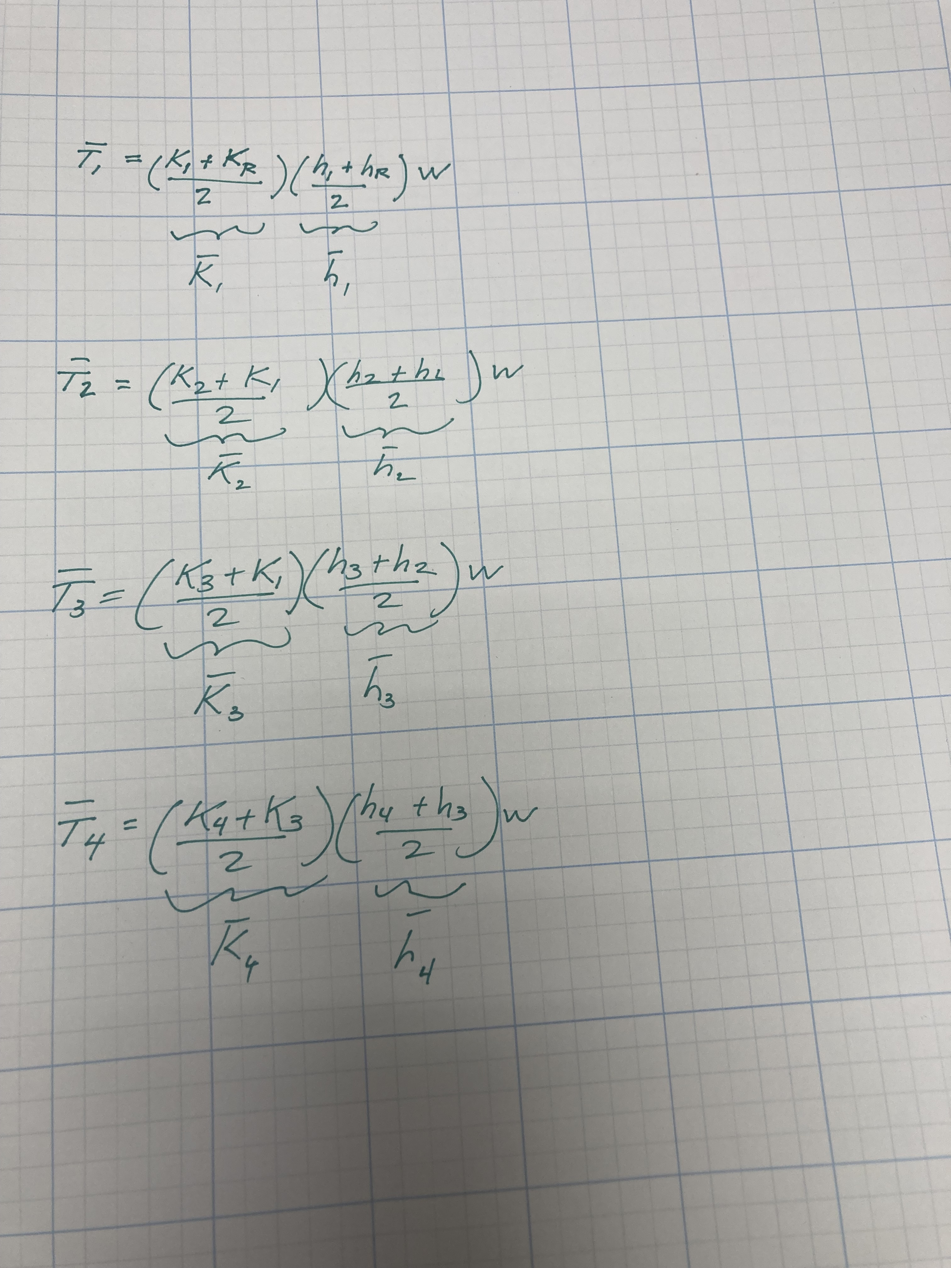
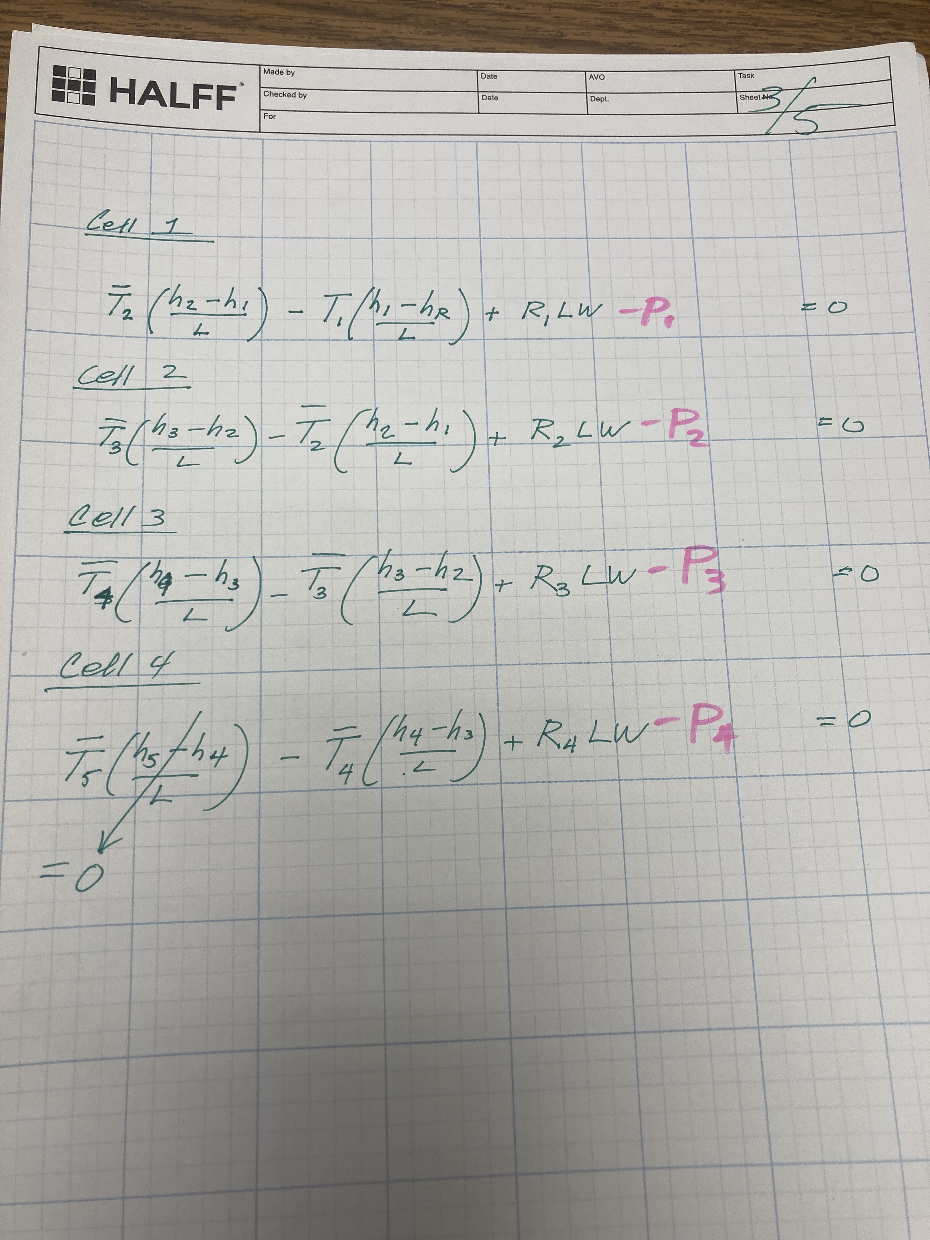
- Write the steady-flow balance equations to estimate average water levels in the four cells.
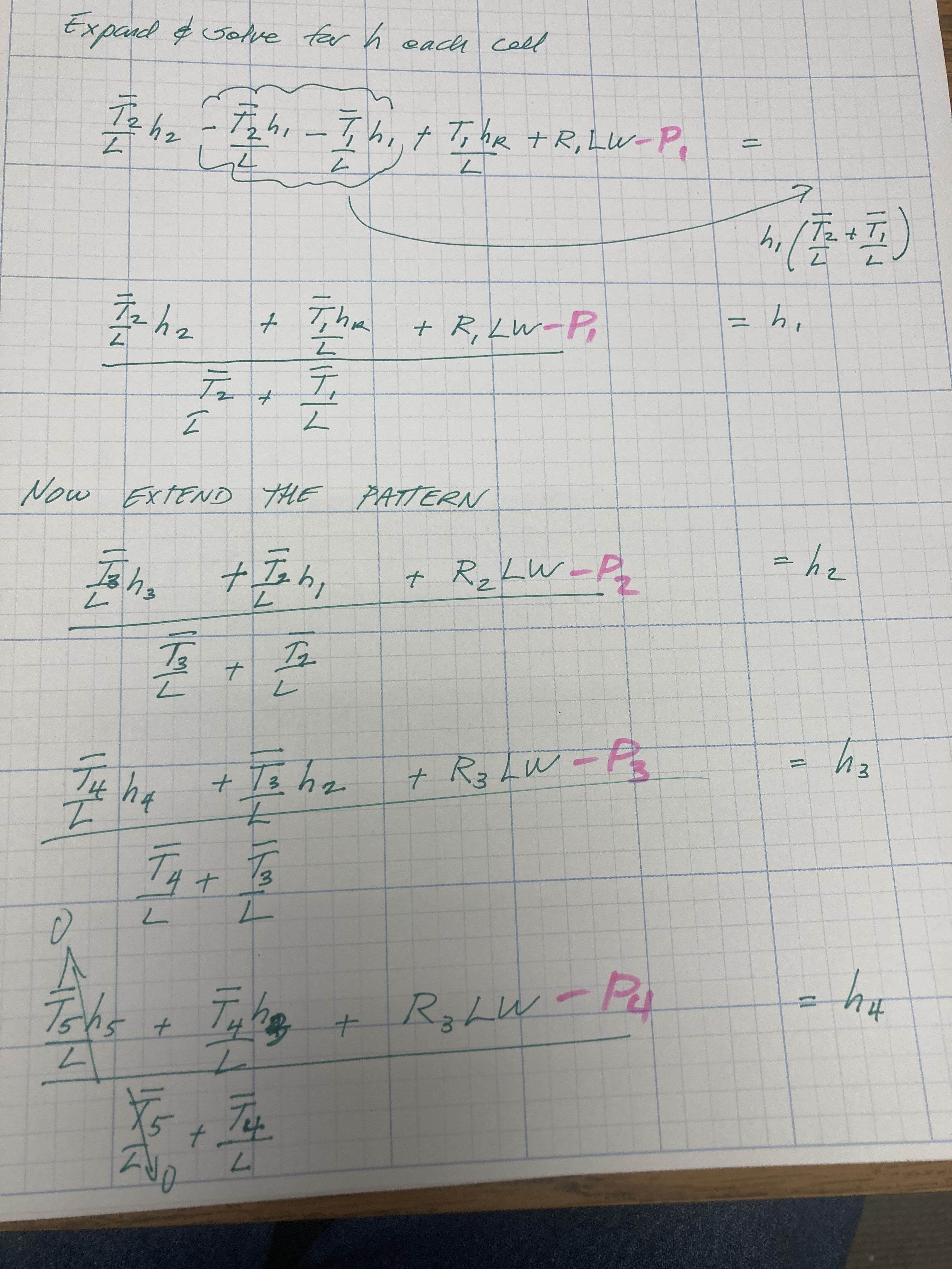
- Solve these equations to determine the average elevations in the 4 cells without pumping.
- Solve these equations when pumping takes place in Cells 2 and 3 at rates of $4\times10^{6}~\frac{m^3}{yr}$ and $7\times10^{6}~\frac{m^3}{yr}$, respectively.
Reference(s)
- Bear (1979). Hydraulics of Groundwater McGraw-Hill (Chapter 10: Modeling of Aquifer Systems) (Eq. 10-9) is useful.
1. Write the steady-flow balance equations to estimate average water levels in the four cells.
2. Solve these equations to determine the average elevations in the 4 cells without pumping.
# No pumping

# STEP 1
KR=3*365 # RIVER CELL
K1=3*365
K2=3*365
K3=6*365
K4=6*365
#
W=3000
L=5000
#
R1=0.4
R2=0.3
R3=0.3
R4=0.2
h=[160,160,160,160,160] # initial guess of heads
hold = h[:]
#
KB1=(K1+KR)*0.5
KB2=(K2+K1)*0.5
KB3=(K3+K2)*0.5
KB4=(K4+K3)*0.5
# INITIAL TRANSMISSIVITY
TB1=KB1*(h[1]+h[0])*0.5*W/L
TB2=KB2*(h[2]+h[1])*0.5*W/L
TB3=KB3*(h[3]+h[2])*0.5*W/L
TB4=KB4*(h[4]+h[3])*0.5*W/L

for updates in range(100): # do a bunch of updates
    h = hold[:]
    for iter in range(100): # do a bunch of iterations per update
        h[1]=(TB2*h[2]+TB1*h[0]+R1*W*L)/(TB2+TB1)
        h[2]=(TB3*h[3]+TB2*h[1]+R2*W*L)/(TB3+TB2)
        h[3]=(TB4*h[4]+TB3*h[2]+R3*W*L)/(TB4+TB3)
        h[4]=(         TB4*h[3]+R4*W*L)/(TB4    )
    hold = h[:]
# update the transmissivity array
    TB1=KB1*(hold[1]+hold[0])*0.5*W/L
    TB2=KB2*(hold[2]+hold[1])*0.5*W/L
    TB3=KB3*(hold[3]+hold[2])*0.5*W/L
    TB4=KB4*(hold[4]+hold[3])*0.5*W/L
print(hold)

# check results
cell1 = TB2*(h[2]-h[1])-TB1*(h[1]-h[0])+R1*W*L
cell2 = TB3*(h[3]-h[2])-TB2*(h[2]-h[1])+R2*W*L
cell3 = TB4*(h[4]-h[3])-TB3*(h[3]-h[2])+R3*W*L
cell4 =                -TB4*(h[4]-h[3])+R4*W*L
bal = [cell1,cell2,cell3,cell4]
print(bal)
# with pumping

# STEP 1
KR=3*365 # RIVER CELL
K1=3*365
K2=3*365
K3=6*365
K4=6*365
#
W=3000
L=5000
#
R1=0.4
R2=0.3
R3=0.3
R4=0.2
h=[160,160,160,160,160] # initial guess of heads
hold = h[:]
#
KB1=(K1+KR)*0.5
KB2=(K2+K1)*0.5
KB3=(K3+K2)*0.5
KB4=(K4+K3)*0.5
# INITIAL TRANSMISSIVITY
TB1=KB1*(h[1]+h[0])*0.5*W/L
TB2=KB2*(h[2]+h[1])*0.5*W/L
TB3=KB3*(h[3]+h[2])*0.5*W/L
TB4=KB4*(h[4]+h[3])*0.5*W/L
# pumping
P1=0
P2=4e6
P3=7e6
P4=0

for updates in range(100): # do a bunch of updates
    h = hold[:]
    for iter in range(100): # do a bunch of iterations per update
        h[1]=(TB2*h[2]+TB1*h[0]+R1*W*L-P1)/(TB2+TB1)
        h[2]=(TB3*h[3]+TB2*h[1]+R2*W*L-P2)/(TB3+TB2)
        h[3]=(TB4*h[4]+TB3*h[2]+R3*W*L-P3)/(TB4+TB3)
        h[4]=(         TB4*h[3]+R4*W*L-P4)/(TB4    )
    hold = h[:]
# update the transmissivity array
    TB1=KB1*(hold[1]+hold[0])*0.5*W/L
    TB2=KB2*(hold[2]+hold[1])*0.5*W/L
    TB3=KB3*(hold[3]+hold[2])*0.5*W/L
    TB4=KB4*(hold[4]+hold[3])*0.5*W/L
print(hold)

# check results
cell1 = TB2*(h[2]-h[1])-TB1*(h[1]-h[0])+R1*W*L-P1
cell2 = TB3*(h[3]-h[2])-TB2*(h[2]-h[1])+R2*W*L-P2
cell3 = TB4*(h[4]-h[3])-TB3*(h[3]-h[2])+R3*W*L-P3
cell4 =                -TB4*(h[4]-h[3])+R4*W*L-P4
bal = [cell1,cell2,cell3,cell4]
print(bal)
Question 4 (30 pts.)
The figure is a plan view of a confined aquifer showing two contaminated zones, 1 and 2. The aquifer has a saturated thickness of 80 ft, hydraulic conductivity of 42 ft/d, and the regional hydraulic gradient is 0.0075 from right to left as shown. A pumping well with a flow rate of 170 gpm is planned to run continuously at the location shown, and form a stable (equilibrium) capture zone. You may assume that the 2500 ft distance from the well to zone 1 is long enough that the capture zone has reached its maximum width.
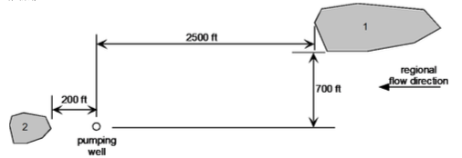
Determine:
- If contamination from zone 1 find its way to the pumping well? Provide support for your answer with a capture zone analysis or contaminant simulation model.
- If contamination from zone 2 find its way to the pumping well? Provide support for your answer with a capture zone analysis or contaminant simulation model.
References
Convert to SI units for Type Curve use:
Q = 170 gpm (1/7.48) (1/3.28)^3 1440 = 927 m^3/day B = 80ft (1/3.28) = 24 meters U = 42 ft/d (1/3.28) = 12.08 m/day 0.0075 = 0.0906
Q/BU for this porblem is 927/(24 * 0.09) = 847
Now plot
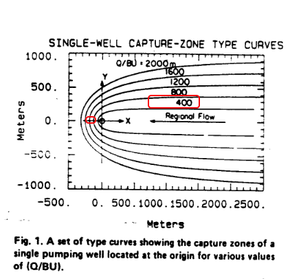
So Zone 1 the elongated rectangle to right side will be captured.
Zone 2 to the left of the well will not.
Obviously, with dimensioned drawings can make point a little better.
CE 5363 Question 5 (30 pts.)
A saturated aquifer sample core of diameter 2.54 cm and length of 6 cm weighs 63 grams. After drying the sample weighs 53 grams. The core sample was placed into an permeameter and exposed to a unit hydraulic gradient. The measured flowrate was 25.4 milliliters/second.
The water levels in three wells in the same aquifer were measured in meters above MSL. The levels were: Well MW-1: 83.1 m; Well MW-2: 84.6 m; Well MW-3: 83.9 m.
Well MW-2 is located 1km due north of Well MW-1, and Well MW-3 is located 700 meters Northeast of Well MW-1.
Determine:
- Estimate the porosity of the aquifer.
- Estimate the hydraulic conductivity of the aquifer.
- Sketch the relative positions of the three wells. Use MW-1 as the origin of the local (your sketch) coordinate system, and North is to the top of your sketch.
- Determine the magniture and direction of the hydraulic gradient in the aquifer monitored by the three wells. Indicate the hydraulic gradient on your sketch (direction and magnitude)
- Estimate the concentration of a conservative constituient (contaminant) at a receptor 4 km away from MW-1 on a flowline that passes through MW-1 using the Ogata-Banks model, assuming MW-1 is at the source location, and the source concentration is 1000 mg/l. Use one-tenth of the path length as the aquifer dispersivity (recall dispersion coefficient is the product of dispersivity and average linear velocity). Calculate the receptor concentration from 0 days after release to 1000 days after release in 10 day increments, and make a concentration history plot for the receptor location.
- An estimate of the time from release until the concentration at the receptor is 500 mg/L.
References
1
Voids = 10 cc. (10 g water)
Volume Bulk = 0.25 pi 2.54^2 * 6 = 30.4 cm^3
n = Voids/Bulk = 10/30.4 = 0.32
2
K = Q/A/grad = 25.4/(0.25 pi 2.54^2) = 5.0 cm/sec
3 and 4
Script below
import numpy
import math
# well A is origin
wellID =['MW1','MW2','MW3']
well_X =[0.0,0.0,494.9]
well_Y =[0.0,1000.0,494.9]
well_Z =[83.1,84.6,83.9]
amatrix = [[0 for j in range(3)]for i in range(3)]
b = [0 for j in range(3)]
# A-matrix
for i in range(3):
    amatrix[i][0]=well_X[i]
    amatrix[i][1]=well_Y[i]
    amatrix[i][2]=1.0
    b[i]= well_Z[i]
amatrix = numpy.array(amatrix) #typecast as numpy array
b = numpy.array(b)
x = numpy.linalg.solve(amatrix,b) # solve equation of plane
# recover and report results
print("x-component hydraulic gradient: ",round(-x[0],3))
print("y-component hydraulic gradient: ",round(-x[1],3))
grad = math.sqrt(x[0]**2+x[1]**2)
print("magnitude hydraulic gradient: ",round(grad,3))
print("direction cosine x-component hydraulic gradient: ",round(-x[0]/grad,3))
print("direction cosine y-component hydraulic gradient: ",round(-x[1]/grad,3))
# use this if want to plot
list1 = [0,-100*x[0]/grad]
list2 = [0,-100*x[1]/grad]
stry='Distance Northing'
strx='Distance Easting'
strtitle='Hydraulic Gradient and 3-Well Locations\n'+'Gradient Magnitude: '+ str(round(grad,3)) +'\n Red segment is 100X direction cosines'

plotlabel=['Wells','Gradient']
from matplotlib import pyplot as plt # import the plotting library from matplotlibplt.show()
plt.plot(well_X, well_Y, color ='green', marker ='o', linestyle ='none') # create a line chart, years on x-axis, gdp on y-axis
plt.plot(list1, list2, color ='red', marker ='x', linestyle ='solid')
plt.title(strtitle)# add a title
plt.ylabel(stry)# add a label to the x and y-axes
plt.xlabel(strx)
plt.legend(plotlabel)
plt.grid()
plt.show() # display the plot

Application of Ogata Banks
Seepage Velocity = K grad = 5.0 cm/sec * 0.002 = 0.01 cm/sec = 864 cm/day = 0.864 m/day
Species velocity = seepage velocity/n = 0.864 m/day / 0.32 = 2.700 m/day
D = disperesivity velocity = 400 2.7 = 1080 m^2/d
from math import sqrt,erf,erfc,exp  # get special math functions
#
# prototype ogatabanks function
#
def ogatabanks(c_source,space,time,dispersion,velocity):
    term1 = erfc(((space-velocity*time))/(2.0*sqrt(dispersion*time)))
    term2 = exp(velocity*space/dispersion)
    term3 = erfc(((space+velocity*time))/(2.0*sqrt(dispersion*time)))
    ogatabanks = c_source*0.5*(term1+term2*term3)
    return(ogatabanks)
#
# example inputs
#
c_source = 1000.0 # source concentration
space = 4000.      # where in X-direction are we
time  = 1000.      # how far in T-direction to extend the plot (change to 1400 for 500 ppm find)
dispersion = 1080.0  # dispersion coefficient
velocity = 2.7    # pore velocity
#
# forward define and initialize vectors for a profile plot
#
how_many_points = 50
deltat = time/how_many_points
t = [i*deltat for i in range(how_many_points)] # constructor notation
c = [0.0 for i in range(how_many_points)]      # constructor notation

t[0]=1e-5 #cannot have zero time, so use really small value first position in list
#
# build the profile predictions
#
for i in range(0,how_many_points,1):
    c[i] = ogatabanks(c_source,space,t[i],dispersion,velocity)
#
# Import graphics routines for picture making
#
from matplotlib import pyplot as plt
#
# Build and Render the Plot
#
plt.plot(t,c, color='red', linestyle = 'solid')  # make the plot object
plt.title(" Concentration History \n Space: " + repr(space) + " space units \n" + " Dispersion: " + repr(dispersion) + " length^2/time units \n" + " Velocity: " + repr(velocity) + " length/time units \n") # caption the plot object
plt.xlabel(" Time since release ") # label x-axis
plt.ylabel(" Concentration        ") # label y-axis
#plt.savefig("ogatabanksplot.png") # optional generates just a plot for embedding into a report
plt.show() # plot to stdio -- has to be last call as it kills prior objects
plt.close('all') # needed when plt.show call not invoked, optional here
#sys.exit() # used to elegant exit for CGI-BIN use

c[-1]
At 1000 days, about 230ppm concentration
Time to 500 ppm is 1400 days
CE 5363 Question 6 (15 pts.)
The three figures below depict streamline patterns for flow near a circular region.
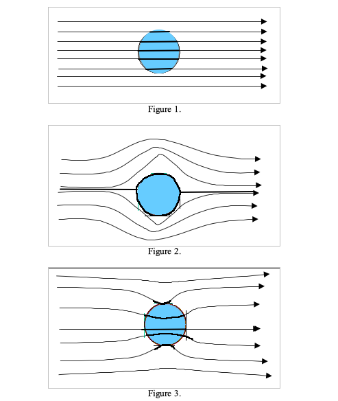
Explain the differences in the patterns in terms of the hydraulic conductivity within the circular region and the surrounding region.
- Circle same K as surround
- Circle smaller K than surround, flow moves around object
- Circle larger K than surround, flow "drawn into" region by low permeability
CE 4363/5363 Question 7 (Extra Credit) (10 pts.)
Consider a single “cell” model. The cell contains a liquid with known initial concentration of a pollutant. The cell is flushed at a constant flow rate with a liquid with zero concentration of the pollutant.
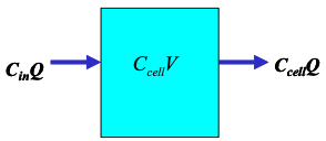
The cell is completely back-mixed, so any mass entering is uniformily distributed within the cell. The volume of the cell is $V$, the discharge entering and leaving is $Q$
Determine:
- An expression for the mass of pollutant in the cell at any time.
- A difference expression for the change in mass in the cell over a discrete time interval (∆t).
- The mass flow of pollutant into the cell (yes, I know its zero, but play along).
- The mass flow of pollutant leaving the cell.
- Combine 2,3, and 4 into a single balance expression (i.e. $\frac{\Delta C}{\Delta t} = \dots~$).