Exercise 4-1 (Problem ?? pp. ??)
The Theis (Eqn. 5.12, p. 162) and Cooper-Jacob (Eqn. 5.54 p. 180) equations can both be used to estimate drawdown for confined aquifer transient problems. A fully penetrating pumping well flows at 300 gpm in a confined aquifer with transmissivity of 11,500 gpd/ft and storage coefficient of 0.00043.
The two models are:
- Theis: $s(r,t) = \frac{Q_w}{4 \pi T}W(u)$
- Cooper-Jacob: $s(r,t) = \frac{Q_w}{4 \pi T}[-0.5772-ln(u)]$
where $u=\frac{r^2 S}{4 T t}$
Determine:
- The drawdown at an observation well 125 ft from the pumping well at 3 hr after pumping started using the Theis solution.
- The drawdown at an observation well 125 ft from the pumping well at 3 hr after pumping started using the Cooper-Jacob simplification.
- For this distance of 125 ft, at what time value in hours does u=0.01?
# Build Computation Tools:

def W(u): # Theis well function using exponential integral
    import scipy.special as sc
    w = sc.expn(1,u)
    return(w)

def ddn_theis(radius,time,storage,transmissivity,discharge): # Drawdown function using exponential integral
    import math
    u = ((radius**2)*(storage))/(4*transmissivity*time)
    s = ((discharge)/(4*math.pi*transmissivity))*W(u)
    return(s)

def ddn_jacob(radius,time,storage,transmissivity,discharge): # Drawdown function using jacob approximation
    import math
    u = ((radius**2)*(storage))/(4*transmissivity*time)
    s = ((discharge)/(4*math.pi*transmissivity))*(-0.5772 - math.log(u))
    return(s)
# Part 1
radius = 125
transmissivity = 11500 # gpd/ft (need to convert to ft^2/day)
transmissivity = transmissivity*(1/7.485) # gpd/7.48g/ft3/ft ->ft^3/day/ft -> ft^2/day! yay!
storage = 0.00043
discharge = 300 #gpm, convert to ft^3/day
discharge = discharge*(1/7.485)*(1440) # gpm/7.48g/ft3 -> ft3/min*1440min/day -> ft3/day
time = 3/24
# all units should be consistent so use the functions
theis = ddn_theis(radius,time,storage,transmissivity,discharge)
print("Drawdown by Theis Solution")
print("Distance to Pumping Well:",round(radius,2)," feet")
print("Pumping Duration:",round(time,2)," days")
print("Transmissivity:",round(transmissivity,2)," sq.ft./day")
print("Storativity:",round(storage,6))
print("Pump Rate",round(discharge,2)," cu.ft./day")
print("Drawdown at Observation Well:",round(theis,2)," feet")
# Part 2
radius = 125
transmissivity = 11500 # gpd/ft (need to convert to ft^2/day)
transmissivity = transmissivity*(1/7.485) # gpd/7.48g/ft3/ft ->ft^3/day/ft -> ft^2/day! yay!
storage = 0.00043
discharge = 300 #gpm, convert to ft^3/day
discharge = discharge*(1/7.485)*(1440) # gpm/7.48g/ft3 -> ft3/min*1440min/day -> ft3/day
time = 3/24
# all units should be consistent so use the functions
jacob = ddn_jacob(radius,time,storage,transmissivity,discharge)
print("Drawdown by Jacob Approximation")
print("Distance to Pumping Well:",round(radius,2)," feet")
print("Pumping Duration:",round(time,2)," days")
print("Transmissivity:",round(transmissivity,2)," sq.ft./day")
print("Storativity:",round(storage,6))
print("Pump Rate",round(discharge,2)," cu.ft./day")
print("Drawdown at Observation Well:",round(jacob,2)," feet")
# Part 3
# Code up the formula then trial-error to fund time that makes u = 0.01
# Or use bisection, quasi-newton, secant ... search methods.  Trial-error probably fastest in terms of human time
# Or use algebra

# By dumbassedry trial-error
time = 0.109326  #guess this value
u = ((radius**2)*(storage))/(4*transmissivity*time)
print("For time:",round(time,6)," value of u is:",round(u,3))
# using algerbra
target = 0.01
time = ((radius**2)*(storage))/(target*4*transmissivity)
print("For time:",round(time,6)," value of u is:",round(target,3))
Exercise 4-2 (Problem ?? pp. ??)
Show how variations in $T$ and $S$ affect transient drawdown curves in an ideal confined aquifer at r = 1, 5, 10, 15, 30, 60, 90, and 120 m when Q = 10 $\frac{L}{sec}$ and t = 400 min.
Determine:
- For $S=5 \times 10^{-4}$ , plot drawdown vs. r for $T=1.0 \times 10^{-1}$ , $1.0 \times 10^{-2}$ , and $1.0 \times 10^{-3}$ $\frac{m^2}{sec}$ on one graph.
- For $T=1.0 \times 10^{-2}$ $\frac{m^2}{sec}$, plot drawdown vs. r for $S=5 \times 10^{-3}$ , $5 \times 10^{-4}$ , and $5 \times 10^{-5}$ on one graph.
- Summarize your findings into a narrative form (e.g. use words)
# Use scripts above, but add some graphics
ttime = 400 # minutes
ttime = 400*60 # convert to seconds

data = \
[[ttime,1],
[ttime ,5],
[ttime ,10],
[ttime ,15],
[ttime ,30],
[ttime ,60],
[ttime ,90],
[ttime ,120]]
S1 = 0.005 # given
S2 = 0.0005
S3 = 0.00005
T1 = 0.1 # given
T2 = 0.01
T3 = 0.001
QLPS = 10 # given
QCMS = QLPS/1000 # convert to LPS to CMS
ddn1 = [0 for i in range(len(data))]
ddn2 = [0 for i in range(len(data))]
ddn3 = [0 for i in range(len(data))]
time = [0 for i in range(len(data))]
distance = [0 for i in range(len(data))]
#print("Time(days)|Radius(ft)|Drawdown(ft)|")
for irow in range(len(data)):
    time[irow]=data[irow][0]
    distance[irow]=data[irow][1]
    ddn1[irow] = ddn_theis(distance[irow],time[irow],S2,T1,QCMS)
    ddn2[irow] = ddn_theis(distance[irow],time[irow],S2,T2,QCMS)
    ddn3[irow] = ddn_theis(distance[irow],time[irow],S2,T3,QCMS)
#    print("%10i|%10i|%12.2f|"%(time[irow],distance[irow],round(ddn3[irow],2)))

# import the package
import matplotlib.pyplot as plt
graph, (plot1) = plt.subplots(1, 1) # create a 1X1 plotting frame
# Code adapted from: https://www.geeksforgeeks.org/how-to-reverse-axes-in-matplotlib/
plot1.plot(distance, ddn1, c='red', marker='x',linewidth=1) # basic line plot
plot1.plot(distance, ddn2, c='green', marker='x',linewidth=1) # basic line plot
plot1.plot(distance, ddn3, c='blue', marker='x',linewidth=1) # basic line plot
#plot1.set_xscale('log') # set x-axis to display a logarithmic scale #################
plot1.set_ylim([0,10])
plot1.invert_yaxis()
plot1.set_xlabel('Distance (m)') # label the x-axis
plot1.set_ylabel('Drawdown (m)') # label the y-axis, notice the LaTex markup
plot1.legend(['T = 0.1','T = 0.01','T = 0.001']) # legend for each series
plot1.set_title('Drawdown vs Distance for S =' + str(round(S2,5))+ '\n') # make a plot title
plot1.grid() # display a grid
plt.show() # display the plot
# Use scripts above, but add some graphics
ttime = 400 # minutes
ttime = 400*60 # convert to seconds

data = \
[[ttime,1],
[ttime ,5],
[ttime ,10],
[ttime ,15],
[ttime ,30],
[ttime ,60],
[ttime ,90],
[ttime ,120]]
S1 = 0.005 # given
S2 = 0.0005
S3 = 0.00005
T1 = 0.1 # given
T2 = 0.01
T3 = 0.001
QLPS = 10 # given
QCMS = QLPS/1000 # convert to LPS to CMS
ddn1 = [0 for i in range(len(data))]
ddn2 = [0 for i in range(len(data))]
ddn3 = [0 for i in range(len(data))]
time = [0 for i in range(len(data))]
distance = [0 for i in range(len(data))]
#print("Time(days)|Radius(ft)|Drawdown(ft)|")
for irow in range(len(data)):
    time[irow]=data[irow][0]
    distance[irow]=data[irow][1]
    ddn1[irow] = ddn_theis(distance[irow],time[irow],S1,T2,QCMS)
    ddn2[irow] = ddn_theis(distance[irow],time[irow],S2,T2,QCMS)
    ddn3[irow] = ddn_theis(distance[irow],time[irow],S3,T2,QCMS)
#    print("%10i|%10i|%12.2f|"%(time[irow],distance[irow],round(ddn3[irow],2)))

# import the package
import matplotlib.pyplot as plt
graph, (plot1) = plt.subplots(1, 1) # create a 1X1 plotting frame
# Code adapted from: https://www.geeksforgeeks.org/how-to-reverse-axes-in-matplotlib/
plot1.plot(distance, ddn1, c='red', marker='x',linewidth=1) # basic line plot
plot1.plot(distance, ddn2, c='green', marker='x',linewidth=1) # basic line plot
plot1.plot(distance, ddn3, c='blue', marker='x',linewidth=1) # basic line plot
#plot1.set_xscale('log') # set x-axis to display a logarithmic scale #################
plot1.set_ylim([0,10])
plot1.invert_yaxis()
plot1.set_xlabel('Distance (m)') # label the x-axis
plot1.set_ylabel('Drawdown (m)') # label the y-axis, notice the LaTex markup
plot1.legend(['S = 0.005','S = 0.0005','S = 0.00005']) # legend for each series
plot1.set_title('Drawdown vs Distance for T =' + str(round(T2,5))+ '\n') # make a plot title
plot1.grid() # display a grid
plt.show() # display the plot
Observe plots far less sensitive to changes in S than changes in T, thus estimates for S need only be sort of close, but estimates of T need to be very close to "truth" to design pumping systems that are effective.
Exercise 4-3 (Problem ?? pp. ??)
A single ideal pumping well, with radius of 1.0 ft and flow rate of 155 gpm, exists in an ideal confined aquifer. The aquifer has a saturated thickness of 82 ft. The pump continues running until equilibrium conditions are reached. The drawdown at the pumping well is 42 ft, and the drawdown at an observation well 138 ft away is 7.5 ft.
Determine:
- Find the transmissivity in $\frac{ft^2}{d}$ and hydraulic conductivity in $\frac{ft^2}{d}$.
- Find the radius of influence in feet.
# Use Theim Solution
# h2-h1 = Q/(2piT)ln(r2/r1)
import math
QGPM = 155 # given
QCFS = QGPM*(1/7.485)*(1440) # convert GPM to CFS
ddn2 = 7.5
ddn1 = 42.0
r2 = 138
r1 = 1
target = ddn1-ddn2 #why -> h1 = ho-ddn1, h2 = ho-ddn2
Tguess = [500,600,700,800,900,1000]
for i in range(len(Tguess)):
    model = (QCFS/(2.0*math.pi*Tguess[i]))*math.log(r2/r1)
    print("T_guess: ",Tguess[i],"Target: ",target," Model: ",model," Error: ",target-model)
So T is somewhere between 600 and 700, refine the search:
# Use Theim Solution
# h2-h1 = Q/(2piT)ln(r2/r1)
import math
QGPM = 155 # given
QCFS = QGPM*(1/7.485)*(1440) # convert GPM to CFS
ddn2 = 7.5
ddn1 = 42.0
r2 = 138
r1 = 1
target = ddn1-ddn2 #why -> h1 = ho-ddn1, h2 = ho-ddn2
Tguess = [600,620,640,660,680,700]
for i in range(len(Tguess)):
    model = (QCFS/(2.0*math.pi*Tguess[i]))*math.log(r2/r1)
    print("T_guess: ",Tguess[i],"Target: ",target," Model: ",model," Error: ",target-model)
Refine again!
# Use Theim Solution
# h2-h1 = Q/(2piT)ln(r2/r1)
import math
QGPM = 155 # given
QCFS = QGPM*(1/7.485)*(1440) # convert GPM to CFS
ddn2 = 7.5
ddn1 = 42.0
r2 = 138
r1 = 1
target = ddn1-ddn2 #why -> h1 = ho-ddn1, h2 = ho-ddn2
Tguess = [677,677.2,677.4,677.6,677.8,678]
for i in range(len(Tguess)):
    model = (QCFS/(2.0*math.pi*Tguess[i]))*math.log(r2/r1)
    print("T_guess: ",Tguess[i],"Target: ",target," Model: ",model," Error: ",target-model)
Klose enough, declare $T = 677.8 \frac{ft^2}{day}$,$K = 677.8/82 = 8.26 \frac{ft}{day}$
The next part is to find r2 so that ddn2 = 0
# Use Theim Solution
# h2-h1 = Q/(2piT)ln(r2/r1)
import math
QGPM = 155 # given
QCFS = QGPM*(1/7.485)*(1440) # convert GPM to CFS
ddn2 = 0 #looking for r2 tro make this happen
ddn1 = 42.0
#r2 = 138
r1 = 1
target = ddn1-ddn2 #why -> h1 = ho-ddn1, h2 = ho-ddn2
Tguess = 677.8
r2 = [340,350,360,370,380,390,400,410]
for i in range(len(r2)):
    model = (QCFS/(2.0*math.pi*Tguess))*math.log(r2[i]/r1)
    print("R_guess: ",r2[i],"Target: ",target," Model: ",model," Error: ",target-model)
So between 400 and 410; refine:
# Use Theim Solution
# h2-h1 = Q/(2piT)ln(r2/r1)
import math
QGPM = 155 # given
QCFS = QGPM*(1/7.485)*(1440) # convert GPM to CFS
ddn2 = 0 #looking for r2 tro make this happen
ddn1 = 42.0
#r2 = 138
r1 = 1
target = ddn1-ddn2 #why -> h1 = ho-ddn1, h2 = ho-ddn2
Tguess = 677.8
r2 = [400,401,402,403,404,405,406,407,408,409,410]
for i in range(len(r2)):
    model = (QCFS/(2.0*math.pi*Tguess))*math.log(r2[i]/r1)
    print("R_guess: ",r2[i],"Target: ",target," Model: ",model," Error: ",target-model)
# Use Theim Solution
# h2-h1 = Q/(2piT)ln(r2/r1)
import math
QGPM = 155 # given
QCFS = QGPM*(1/7.485)*(1440) # convert GPM to CFS
ddn2 = 0 #looking for r2 tro make this happen
ddn1 = 42.0
#r2 = 138
r1 = 1
target = ddn1-ddn2 #why -> h1 = ho-ddn1, h2 = ho-ddn2
Tguess = 677.8
r2 = [402,402.1,402.2,402.3,402.4,402.5,402.6,402.7,402.8,402.9,403]
for i in range(len(r2)):
    model = (QCFS/(2.0*math.pi*Tguess))*math.log(r2[i]/r1)
    print("R_guess: ",r2[i],"Target: ",target," Model: ",model," Error: ",target-model)
So $r=402.7$ is close enough, thus the anticipaed radius of influence is $R_e = 402.7 ~m$
Useful References for Problems below:
- Fetter and Kreamer (2022) Applied Hydrology 5ed. pp. 212-215
- Kelvin's Method of Images for potential flow (MIT fluid flow lecture)
- Method of Images (Wikipedia)
- Carslaw and Jaeger (1959), Conduction of Heat in Solids, 2ed. Oxford University Press in particular Chapter 10 pp. 274
Exercise 4-4 (Problem ?? pp. ??)
An unconfined aquifer exists where a buried river channel cut into underlying impermeable bedrock. The figure below shows the orientation and pertinent dimensions. The flow rate at the pumping well is 250 gpm, and its radius of influence is 1000 ft. The hydraulic conductivity of the aquifer is 15 ft/d, and the initial saturated thickness is 120 ft. Find the drawdown at the observation well under equilibrium conditions.
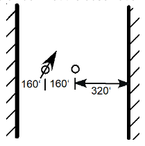
Solution
For any single well:
$s(r,R_{eff})=H_{ref} - \sqrt{[H_{ref}^2 - \frac{Q}{\pi*K}ln(\frac{R_{eff}}{r})]}$
Supoertposition of image wells to complete estimate and reflect boundaries as below:
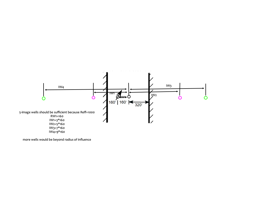
A script for the gonculations:
# model
def head_unconf(radius,discharge,conductivity,href,Reff):
    import math
    if radius >= Reff:
        head_unconf = math.sqrt(href**2 - 0)
    else:
        head_unconf = math.sqrt(href**2 - (discharge/(math.pi*conductivity))*math.log(Reff/radius))
    return(head_unconf)
# parameters
K=15 #ft/day
QGPM = 250 # given
QCFS = QGPM*(1/7.485)*(1440) # convert GPM to CFS
REFF = 1000 #given
HREFF = 120 #given

# ddn from real well
ddn1 = HREFF - head_unconf(160,QCFS,K,HREFF,REFF)
# ddn 1st image
ddn2 = HREFF - head_unconf(3*160,QCFS,K,HREFF,REFF)
# ddn 2nd image
ddn3 = HREFF - ddn_unconf(5*160,QCFS,K,HREFF,REFF)
# ddn 3rd image
ddn4 = HREFF - ddn_unconf(7*160,QCFS,K,HREFF,REFF)
# ddn 4th image
ddn5 = HREFF - ddn_unconf(9*160,QCFS,K,HREFF,REFF)

ddn_obs=ddn1+ddn2+ddn3+ddn4+ddn5

print("Drawdown at observation well from pumping and boundaries: ",round(ddn_obs,3)," feets")
Exercise 4-5 (Problem ?? pp. 216)
Consider the figure below. Wells 1, 2, and 3 are pumping wells, and Obs 1 and 2 are just observation wells (no pumping at all). Provide a sketch to scale, drawn with a straightedge, that shows all the proper image wells (pp. 212-215) necessary to represent the impacts of the two boundaries on the pumping and observation well drawdowns.
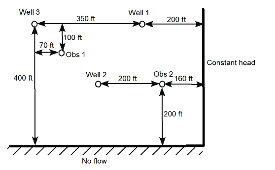
Solution
Create the wellfield array:
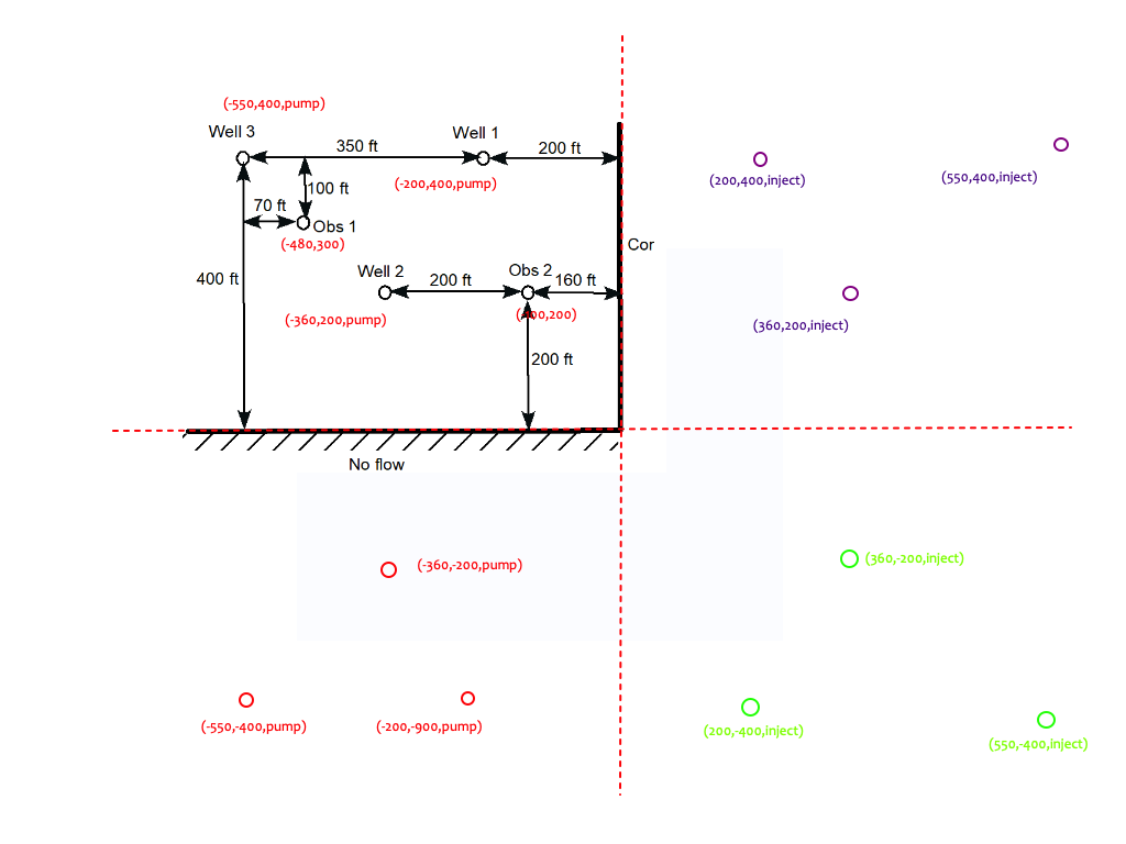
Code the Solution (future exercise)
def W(u): # Theis well function using exponential integral
    import scipy.special as sc
    w = sc.expn(1,u)
    return(w)

def ddn_theis(radius,time,storage,transmissivity,discharge): # Drawdown function using exponential integral
    import math
    u = ((radius**2)*(storage))/(4*transmissivity*time)
    s = ((discharge)/(4*math.pi*transmissivity))*W(u)
    return(s)

# array for observations

# array for pumps

# compute distance
# radius = sqrt(x1-xo**2 +y1-yo**2) ....
Exercise 4-6 (CE 5363 students)(Problem ?? pp. ??)
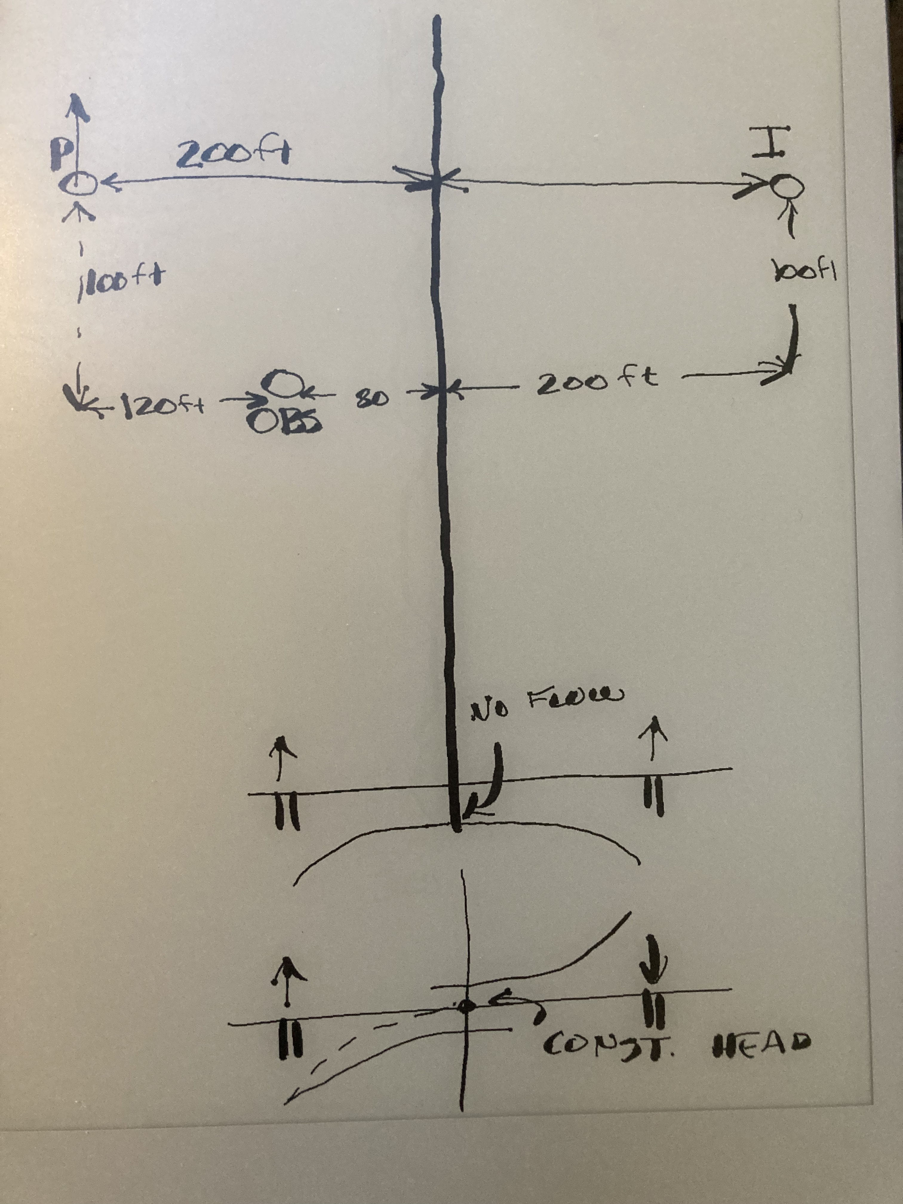
A single pumping well, with a flow rate of 250 gpm, fully penetrates a confined aquifer. The aquifer has a saturated thickness of 110 ft, hydraulic conductivity of 20 ft/d, and storage coefficient of 0.00050. Due to outcropping of the aquifer, a no-flow zone exists 200 ft east of the pumping well and extends as a straight line to both north and south. An observation well is located 100 ft south and 120 ft east of the pumping well.
Determine:
- Drawdown in feet at the observation well at time t=1, 5, 10, 20, 30, 40, 60, 80, 100, 120, 240, 480, 600, 720, 840, 960, 1200, and 1440 min after the well is turned on.
- Plot the drawdown vs. log time.
- Change the boundary type to a constant head boundary and plot the drawdown vs. log time.
- Combine the two plots into a single graph (both boundary types - same graphic)
- Summarize your findings in a narrative (e.g. use words).
Solution
Use tools above, need geometry
# Build Computation Tools:

def W(u): # Theis well function using exponential integral
    import scipy.special as sc
    w = sc.expn(1,u)
    return(w)

def ddn_theis(radius,time,storage,transmissivity,discharge): # Drawdown function using exponential integral
    import math
    u = ((radius**2)*(storage))/(4*transmissivity*time)
    s = ((discharge)/(4*math.pi*transmissivity))*W(u)
    return(s)

import math
QGPM = 250 #given
QCFD = (QGPM/7.48)*1440 #convert gpm to ft^3/day
dpw2obs = math.sqrt(100**2 + 120**2) # pump well to obs
diw2obs = math.sqrt(100**2 + 280**2) # image well to obs
time =[1,5,10,20,30,40,60,80,100,120,240,480,600,720,840,960,1200,1440] # list of times in minuten
for i in range(len(time)):
    time[i]=time[i]/1440.  # convert time into days
K = 20 # hydraulic conductivity in ft/day
b = 110 # aquifer thickness in ft
T = K*b # transmissivity in ft^2/day
S = 0.00050 #given
ddn1 = [0 for i in range(len(time))]
ddnpw = [0 for i in range(len(time))]
ddniw = [0 for i in range(len(time))] # empty vectors to store results
for i in range(len(time)):
    ddnpw[i]=ddn_theis(dpw2obs,time[i],S,T,QCFD)
    ddniw[i]=ddn_theis(diw2obs,time[i],S,T,QCFD)
    ddn1[i]=ddnpw[i]+ddniw[i]

#convert time back to minutes
for i in range(len(time)):
    time[i]=time[i]*1440.  # convert time into minutes
# plot results

# import the package
import matplotlib.pyplot as plt
graph, (plot1) = plt.subplots(1, 1) # create a 1X1 plotting frame
# Code adapted from: https://www.geeksforgeeks.org/how-to-reverse-axes-in-matplotlib/
plot1.plot(time, ddn1, c='red', marker='x',linewidth=1) # basic line plot
#plot1.plot(time, ddnpw, c='green', marker='x',linewidth=1) # basic line plot
#plot1.plot(time, ddniw, c='blue', marker='x',linewidth=1) # basic line plot
plot1.set_xscale('log') # set x-axis to display a logarithmic scale #################
plot1.set_ylim([0,20])
plot1.invert_yaxis()
plot1.set_xlabel('Time (minutes)') # label the x-axis
plot1.set_ylabel('Drawdown (ft)') # label the y-axis, notice the LaTex markup
plot1.legend(['Observed Drawdown','Drawdown from Pumping Well','Drawdown from Image Well']) # legend for each series
plot1.set_title('Drawdown vs Time\n') # make a plot title
plot1.grid() # display a grid
plt.show() # display the plot
# Build Computation Tools:

def W(u): # Theis well function using exponential integral
    import scipy.special as sc
    w = sc.expn(1,u)
    return(w)

def ddn_theis(radius,time,storage,transmissivity,discharge): # Drawdown function using exponential integral
    import math
    u = ((radius**2)*(storage))/(4*transmissivity*time)
    s = ((discharge)/(4*math.pi*transmissivity))*W(u)
    return(s)
import math
QGPM = 250 #given
QCFD = (QGPM/7.48)*1440 #convert gpm to ft^3/day
dpw2obs = math.sqrt(100**2 + 120**2) # pump well to obs
diw2obs = math.sqrt(100**2 + 280**2) # image well to obs
# To change boundary type change sense of pumping on image well
time =[1,5,10,20,30,40,60,80,100,120,240,480,600,720,840,960,1200,1440] # list of times in minuten
for i in range(len(time)):
    time[i]=time[i]/1440.  # convert time into days
K = 20 # hydraulic conductivity in ft/day
b = 110 # aquifer thickness in ft
T = K*b # transmissivity in ft^2/day
S = 0.00050 #given
ddn2 = [0 for i in range(len(time))]
ddnpw = [0 for i in range(len(time))]
ddniw = [0 for i in range(len(time))] # empty vectors to store results
for i in range(len(time)):
    ddnpw[i]=ddn_theis(dpw2obs,time[i],S,T,QCFD)
    ddniw[i]=ddn_theis(diw2obs,time[i],S,T,-QCFD)###########change is here!
    ddn2[i]=ddnpw[i]+ddniw[i]

#convert time back to minutes
for i in range(len(time)):
    time[i]=time[i]*1440.  # convert time into minutes
# plot results

# import the package
import matplotlib.pyplot as plt
graph, (plot1) = plt.subplots(1, 1) # create a 1X1 plotting frame
# Code adapted from: https://www.geeksforgeeks.org/how-to-reverse-axes-in-matplotlib/
plot1.plot(time, ddn2, c='red', marker='x',linewidth=1) # basic line plot
#plot1.plot(time, ddnpw, c='green', marker='x',linewidth=1) # basic line plot
#plot1.plot(time, ddniw, c='blue', marker='x',linewidth=1) # basic line plot
plot1.set_xscale('log') # set x-axis to display a logarithmic scale #################
plot1.set_ylim([0,20])
plot1.invert_yaxis()
plot1.set_xlabel('Time (minutes)') # label the x-axis
plot1.set_ylabel('Drawdown (ft)') # label the y-axis, notice the LaTex markup
plot1.legend(['Observed Drawdown','Drawdown from Pumping Well','Drawdown from Image Well']) # legend for each series
plot1.set_title('Drawdown vs Time\n') # make a plot title
plot1.grid() # display a grid
plt.show() # display the plot
# Now both plots single graph
# import the package
import matplotlib.pyplot as plt
graph, (plot1) = plt.subplots(1, 1) # create a 1X1 plotting frame
# Code adapted from: https://www.geeksforgeeks.org/how-to-reverse-axes-in-matplotlib/
plot1.plot(time, ddn1, c='red', marker='x',linewidth=1) # basic line plot
plot1.plot(time, ddn2, c='green', marker='x',linewidth=1) # basic line plot
#plot1.plot(time, ddniw, c='blue', marker='x',linewidth=1) # basic line plot
plot1.set_xscale('log') # set x-axis to display a logarithmic scale #################
plot1.set_ylim([0,20])
plot1.invert_yaxis()
plot1.set_xlabel('Time (minutes)') # label the x-axis
plot1.set_ylabel('Drawdown (ft)') # label the y-axis, notice the LaTex markup
plot1.legend(['Drawdown - No Flow Boundary','Drawdown - Constant Head Boundary','Drawdown from Image Well']) # legend for each series
plot1.set_title('Drawdown vs Time\n') # make a plot title
plot1.grid() # display a grid
plt.show() # display the plot