Exercise 2-1 (Problem 4.6 pp. 148)
The liquid pressure in the screen of a piezometer in a saline aquifer is $7.688 \times 10^{5} N/m^2$. The liquid density is 1055 kg/m$^3$ and the temperature is 14$^o$C. The elevation of the piezometer is 45.9 m above MSL.
Determine:
- The point-water pressure head.
- The fresh-water pressure head.
- The total fresh-water head.
Solution:
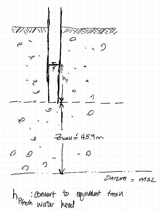
# Point water pressure head
p = 7.688e05 #Pa given
rho = 1055 #kg/m^3 given
g = 9.81 #m/s/s
def headp(pressure,rho,gee):
    headp=pressure/(rho*gee)
    return(headp)
hp=headp(p,rho,g)
print("Point pressure head: ",round(hp,3)," meters")
# Fresh water pressure head
rho_f = 999 # see table lookup next problem, should be at 14C
hpf = hp*rho/rho_f
print("Equivalent fresh water pressure head: ",round(hpf,3)," meters")
# Total fresh water pressure head
zwell = 45.9
hp_total = hpf+zwell
print("Total fresh water pressure head: ",round(hp_total,3)," meters")
Exercise 2-2 (Problem 4.8 pp. 148)
An aquifer has a hydraulic conductivity of 12 ft/day and an effective porosity of 0.17 and is under a hydraulic gradient of 0.0055. The water temperature is 14$^o$C and the mean pore diameter is 0.33 mm.
Determine:
- The specific discharge.
- The average linear velocity.
- If Darcy's law is applicable under these conditions; justify your answer.
Solution:
2-2(1)
$q = K \frac{dh}{dl}$
K = 12 #ft/day
dhdl = 0.0055 #given
q = K*dhdl
print("Specific discharge: ",q," ft/day")
2-2(2)
$v = \frac{q}{n}$
n_e = 0.17 #given
v = q/n_e
print("Average linear velocity: ",round(v,3)," ft/day")
2-2(3)
Is Darcy's law applicable?
Evaluate value of Reynolds' number, Re > 10 is usual rule for invalidity (our book suggests Re > 1 is the magic value) either way we have to evaluate Re.
$Re_d = \frac{\rho q d_{10}}{\mu}$ (Eq 4.20 in the book)
Both $\rho$ and $\mu$ are temperature dependent so need to look up values
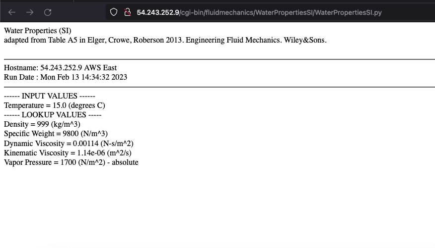
rho = 999 #kg/m^3
mu = 0.00114 #N-s/m^s
D_10 = 0.33e-03 # 0.33mm into meters
q_si = q*(1/3.28)*(1/86400)  #ft/day * (1m/3.28ft)*(1day/86400sec)
Re_d = (rho * q_si * D_10)/(mu)
print("Reynolds Number: ",round(Re_d,6)," ")
$Re_d$ is less than 10 or 1, so Darcy's law valid.
Exercise 2-3 (Problem 4.10 pp. 148)
A confined aquifer is 18 m thick. The potentiometric surface drops 1.99 m between two wells that are 823 m apart. The hydraulic conductivity of the aquifer is 4.35 m/day
Determine:
- Discharge per unit width in the aquifer in cubic meters per day
Solution:
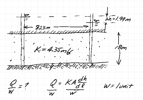
$\frac{Q}{w} = \frac{1}{w} K b w \frac{dh}{dl}$
K = 4.35 #m/day given
b = 18 #m given
w = 1 #m given "unit width"
dh = 1.99 #m given
dl = 823 #m given
Q = K*b*w*(dh/dl)
print("Discharge per unit width: ",round(Q/w,3)," m^2/day")
Exercise 2-4 (Problem 4.13 pp. 149)
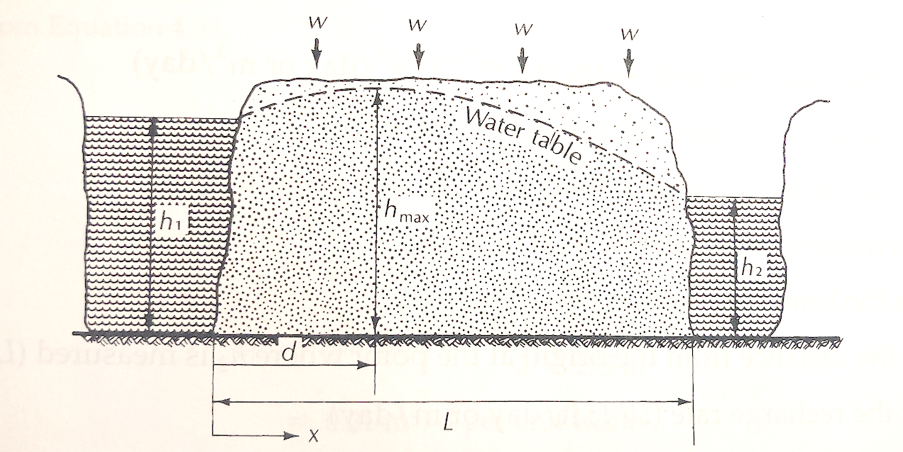
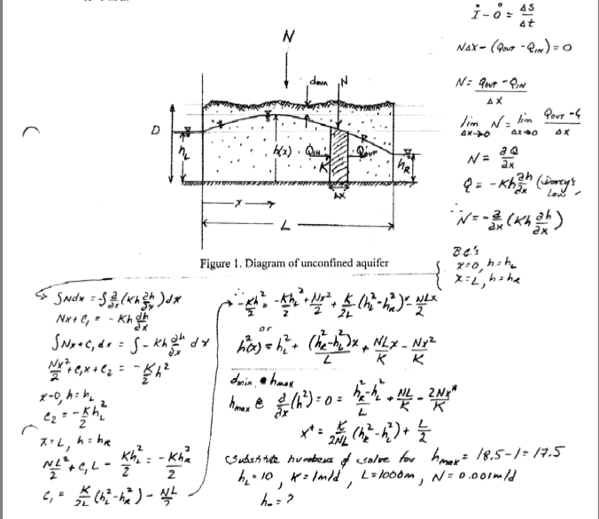
In the figure below (Fig. 4.19) the hydraulic conductivity of the aquifer is 14.5 m/day. The value of $h_1$ is 17.6 m, and the value of $h_2$ is 15.3 m. The distance from $h_1$ to $h_2$ is 525 m. There is an average recharge rate of 0.007 m/day.
Determine:
- The average discharge per unit width at $x=0$.
- The average discharge per unit width at $x=525$.
- The location of the water-table divide (if it exists)
- The maximum height of the water table.
Solution
Need the equation of the water surface for all 4 parts.
hL = 17.6 #m given
hR = 15.3 #m given
N = 0.007 #m/day
K = 14.5 #m/day
xL = 0 #m given
xR = 525 #m given
def h(x,hL,hR,N,K,xL,xR):
    L = xR-xL
    hsq = hL**2 + ((hR**2 - hL**2)*x)/L + (N*L*x)/K - (N*x**2)/K
    h=hsq**(0.5)
    return(h)
- The average discharge per unit width at $x=0$.
Need gradient at x=0 from the right. Approximate using finite-difference as
h0 = h(0,hL,hR,N,K,xL,xR)
h1 = h(1.0,hL,hR,N,K,xL,xR)
dh = h0 - h1
dl = 1.0
print("gradient at x=0: ",round(dh/dl,3))
discharge = h0*K*dh/dl
print("discharge at x=0: ",round(discharge,3),' m^3/day/m')
The negaitve result implies flow is to the left!
- The average discharge per unit width at $x=525$.
Need gradient at x=L from the left. Approximate using finite-difference as
hR_1 = h(xR-1.0,hL,hR,N,K,xL,xR)
dh = hR-hR_1
dl = 1.0
print("gradient at x=0: ",round(-dh/dl,5))
discharge = -hR*K*(dh/dl)
print("discharge at x=xR: ",round(discharge,3),' m^3/day/m')
The positve result implies flow is to the right!
- The location of the water-table divide (if it exists)
The formula is in the graphic above, here we can just plot the function and get close by looking at the plot.
# lists of zeros to store results
xloc = [0 for i in range(100)]
zloc = [hL for i in range(100)]
increment = (xR-xL)/99
for i in range(1,100):
    xloc[i]=xloc[i-1]+increment
    zloc[i]=h(xloc[i],hL,hR,N,K,xL,xR)
stry='Piezometric Surface Elevation (meters)'
strx='Distance (meters)'
strtitle='Plot of Groundwater Surface in Unconfined Aquifer Between two ditches with Recharge'
from matplotlib import pyplot as plt # import the plotting library from matplotlibplt.show()
plt.plot(xloc, zloc, color ='blue', marker ='o', linestyle ='none')
plt.title(strtitle)# add a title
plt.ylabel(stry)# add a label to the x and y-axes
plt.xlabel(strx)
plt.ylim([15,20])
plt.grid()
plt.show() # display the plot
So the peak is at about x=120. Now apply the formula to confirm:
L = xR-xL
xstar = (K)/(2*N*L)*(hR**2 - hL**2)+L/2
print("Water Table Divide Location: ",round(xstar,1)," meters from left drain")
- The maximum height of the water table.
This is simply the head at xstar
print("Maximum height of water table: ",round(h(xstar,hL,hR,N,K,xL,xR),3)," meters")
Exercise 2-5
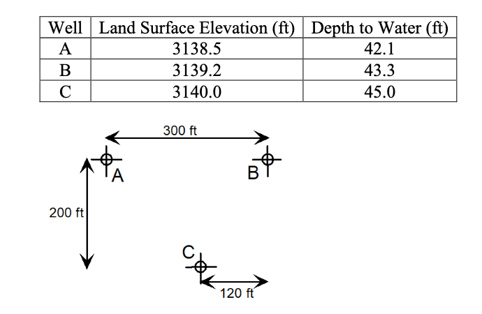
Three monitoring wells exist in an aquifer as shown below. North is upward (toward the top of the page). The land surface elevations and depths to water are shown below.
Determine:
- The magnitude and direction of the head gradient.
Solution:
- Use the graphical method in notes
- Use a spreadsheet (Works in LibreOffice if you supress the Macro and don't use the save and exit button) Model1_Gradient.xls
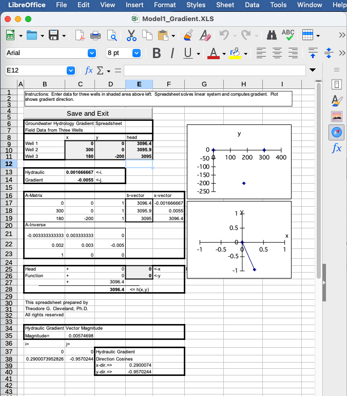
- Solve the equation of the plane through the three wells (Same as the spreadsheet, but using ENGR 1330 methods as shown below)
import numpy
import math
# well A is origin
wellID =['Well A','Well B','Well C']
well_X =[0.0,300.0,180.0]
well_Y =[0.0,0.0,-200.0]
well_Z =[3138.5-42.1,3139.2-43.3,3140.0-45.0]
amatrix = [[0 for j in range(3)]for i in range(3)]
b = [0 for j in range(3)]
# A-matrix
for i in range(3):
    amatrix[i][0]=well_X[i]
    amatrix[i][1]=well_Y[i]
    amatrix[i][2]=1.0
    b[i]= well_Z[i]
amatrix = numpy.array(amatrix) #typecast as numpy array
b = numpy.array(b)
x = numpy.linalg.solve(amatrix,b) # solve equation of plane
# recover and report results
print("x-component hydraulic gradient: ",round(-x[0],3))
print("y-component hydraulic gradient: ",round(-x[1],3))
grad = math.sqrt(x[0]**2+x[1]**2)
print("magnitude hydraulic gradient: ",round(grad,3))
print("direction cosine x-component hydraulic gradient: ",round(-x[0]/grad,3))
print("direction cosine y-component hydraulic gradient: ",round(-x[1]/grad,3))
# use this if want to plot
list1 = [0,-100*x[0]/grad]
list2 = [0,-100*x[1]/grad]
stry='Distance Northing'
strx='Distance Easting'
strtitle='Hydraulic Gradient and 3-Well Locations\n'+'Gradient Magnitude: '+ str(round(grad,3)) +'\n Red segment is 100X direction cosines'

plotlabel=['Wells','Gradient']
from matplotlib import pyplot as plt # import the plotting library from matplotlibplt.show()
plt.plot(well_X, well_Y, color ='green', marker ='o', linestyle ='none') # create a line chart, years on x-axis, gdp on y-axis
plt.plot(list1, list2, color ='red', marker ='x', linestyle ='solid')
plt.title(strtitle)# add a title
plt.ylabel(stry)# add a label to the x and y-axes
plt.xlabel(strx)
plt.legend(plotlabel)
plt.grid()
plt.show() # display the plot