Download (right-click, save target as ...) this page as a Jupyterlab notebook from: ES-3
Problem 1
A subcritical transition from an upstream rectangular flume that is 49 $ft$ wide to a downstream trapezoidal channel with a width of 75 $ft$ and side slopes of 2:1. The transition bottom drops 1 $ft$ from the upstream flume to the downstream trapezoidal channel. The steady discharge is 12,600 $cfs$ and the depth of flow in the downstream channel is 22 $ft$. For a head loss coefficient of 0.5
Determine:
- The approach flow depth (in the rectangular flume).
sketch(s) here
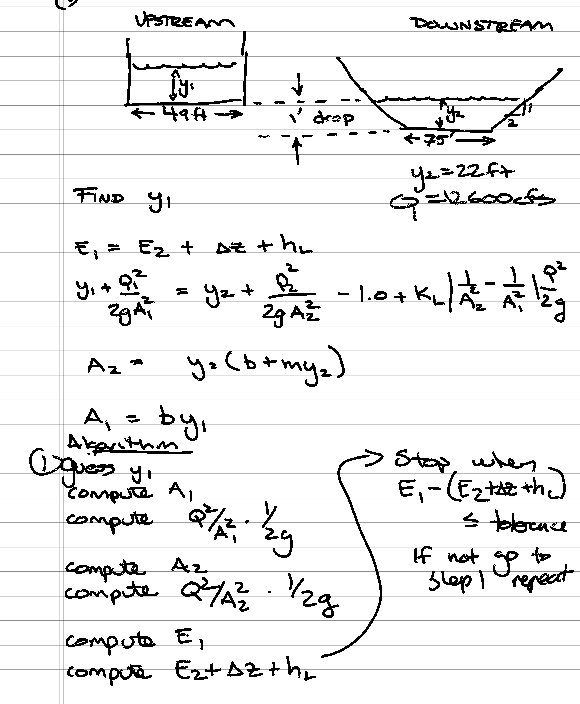
list known quantities
$y_2$
$B_1$
$B_2$
$m$
$Q$
Geometry each section
$\Delta z$
list unknown quantities
- $y_1$
governing principles
- Modified Bernoulli for open channels
# solution (step-by-step/computations)
import math
y1 = 19.880 # <<< Guess and adjust this value
y2 = 22.0 # ft given
Q = 12600 # cfs given
g = 32.2 # ft/s/s given
b1 = 49.0 # given
b2 = 75.0 # given
m2 = 2.0 #given
Dz = -1.0 #given
Kl = 0.5 #given
deltaY = 0.0001
tolerance = 0.0001


for i in range(10000):
    y1 = y1+float(i)*deltaY
    Q2g = (Q**2/(2.0*g))
    A1 = b1*y1
    A2 = y2*(b2+m2*y2)
    E1 = y1 + Q2g/(A1**2)
    E2 = y2 + Q2g/(A2**2)
    LHS = E1
    RHS = E2 + Dz + Kl*abs(1/(A1**2)-1/(A2**2))*Q2g
    if abs(LHS-RHS) <= tolerance:
        print("y1 ",round(y1,3),"y2",round(y2,3)," Energy Error ",round(LHS-RHS,3))
discussion
By a "brute force" search approach depth is 19.881 feet.
Problem 2
A circular culvert with 1.0 $m$ diameter is placed on a steep slope. The upstream head is 1.3 $m$ with an unsubmerged entrance. Neglect entrance losses and
Determine:
- The discharge through the culvert.
- The critical depth at the entrance.
sketch(s) here
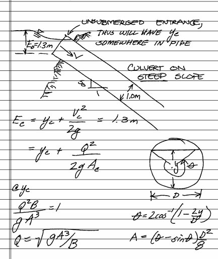
list known quantities
- $E_o$
- Unsubmerged inlet
- Neglect head losses
- Hydraulically steep slope
list unknown quantities
- $y_c$ Just before jump close to inlet most likely
- $Q$
governing principles
- Energy balance, critical energy
- Algebra too!
# prototype functions
def area(theta,diameter):
    import math
    area=(1/8)*(theta-math.sin(theta))*diameter**2
    return(area)

def topw(theta,diameter):
    import math
    topw=diameter*math.sin(theta/2)
    return(topw)

def angle(depth,diameter):
    angle=2*math.acos(1-2*depth/diameter)
    return(angle)

# solution script
import math
g = 9.81
D = 1.0
y = 0.8825  # <<< Guess this value
Ec = 1.3

Q = math.sqrt(g*area(angle(y,D),D)**3/topw(angle(y,D),D))
E = y+Q**2/(2*g*area(angle(y,D),D))
print("Entrance Depth = ",round(y,3)," meters \nDischarge = ",round(Q,3)," m^3/sec \nEnergy Balance Error = ",round(E-Ec,3))
discussion
Brute force, non-elegant, balance two sides of equation by guess-and-check.
Problem 3
A 1.0 $m$ by 1.0 $m$ box culvert is placed on a steep slope. The upstream head is 1.3 $m$ with an unsubmerged entrance. Neglect entrance losses and
Determine:
- The discharge through the culvert.
- The critical depth at the entrance.
sketch(s) here
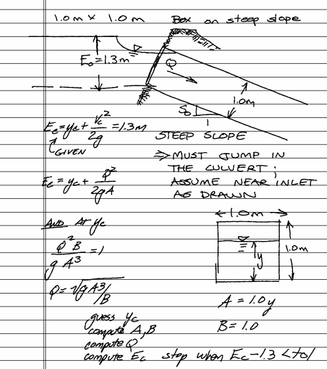
list known quantities
- $E_o$
- Unsubmerged inlet
- Neglect head losses
- Hydraulically steep slope
list unknown quantities
- $y_c$ Just before jump close to inlet most likely
- $Q$
# solution (step-by-step/computations)
# prototype functions
def area(width,depth):
    import math
    area=width*depth
    return(area)

# solution script
import math
g = 9.81
W = 1.0
y = 0.8975 # <<< Guess this value
Ec = 1.3

Q = math.sqrt(g*area(W,y)**3/W)
E = y+Q**2/(2*g*area(W,y))
print("Entrance Depth = ",round(y,3)," meters \nDischarge = ",round(Q,3)," m^3/sec \nEnergy Balance Error = ",round(E-Ec,3))
discussion
Yea, just reuse code, change geometry
Problem 4
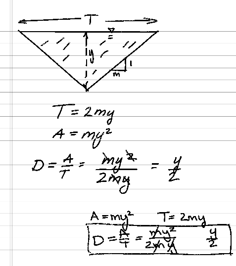
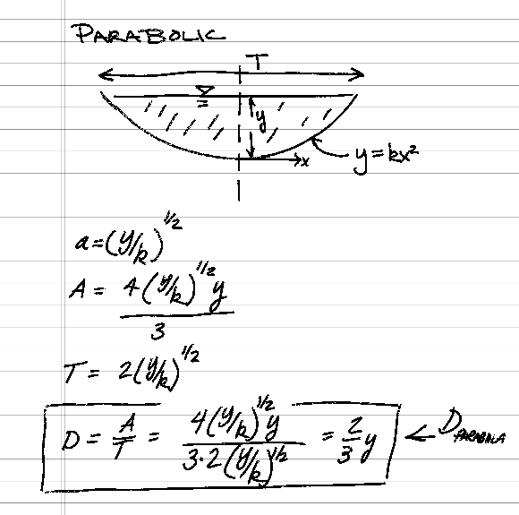
A study of natural channel shapes in the western United States reported an average ratio of maximum depth to hydraulic depth ($D=\frac{A}{T}$) in the main channel (with no overflow) of $\frac{y}{D} = 1.55$ for 761 measurements.
Determine:
- The calculated ratio of maximum depth to hydraulic depth for a triangular channel.
- The calculated ratio of maximum depth to hydraulic depth for a parabolic channel.
- The calculated ratio of maximum depth to hydraulic depth for a rectangular channel.
- The significance of these calculated results to the study's reported average.
- The discharge for a channel at a critical depth of $y=10.0~ft$ if $\frac{y}{D} = 1.55$ and $T=100~ft$.
list known quantities
list unknown quantities
governing principles
Algebra baby!
# solution (step-by-step/computations)
# For bullet items 1-3
# Bullet 4 in discussion below

y = [0 for i in range(100)]
dtrig = [0 for i in range(100)]
dpara = [0 for i in range(100)]
drect = [0 for i in range(100)]
YoverD = [0 for i in range(100)]

sum = 0.0

for i in range(1,100): # 1 to 10 in steps of 0.01
    y[i] = 100.0*float(i/100)
    dtrig[i]=y[i]/(y[i]/2.0)
    dpara[i]=y[i]/(2.0*y[i]/3.00)
    drect[i]=y[i]/(y[i])
    sum +=(dtrig[i]+dpara[i]+drect[i])/3.0

import matplotlib.pyplot # the python plotting library
myfigure = matplotlib.pyplot.figure(figsize = (10,5)) # generate a object from the figure class, set aspect ratio
# Built the plot
matplotlib.pyplot.plot(y, dtrig, color ='blue')
matplotlib.pyplot.plot(y, dpara, color ='red')
matplotlib.pyplot.plot(y, drect, color ='green')
matplotlib.pyplot.xlabel("Depth (y)")
matplotlib.pyplot.ylabel("Depth (y)/Hydraulic Depth (A/T)")
matplotlib.pyplot.title("Hydraulic Depth vs. Thalweg Depth for Different Channel Geometries")
matplotlib.pyplot.legend(["Triangular Channel","Parabolic Channel","Rectangular Channel"])
matplotlib.pyplot.show()


print("Average y/D value all depths, all geometries ",round(sum/100.0,3))
# bullet item 4
import math
g = 32.2
yc = 10
yOd = 1.55
T = 100
D = yc/yOd
A = T*D
Ec = yc+D/2.0
QQ = 2*g*(Ec-yc)*A**2
Q = math.sqrt(QQ)
#Q = math.sqrt(g*(A**3)/T) # or do the algebra
print("Discharge ",round(Q,3)," CFS")
discussion
Average for natural channels is 1.55, so natural channels tend to be close to parabolic (y/D =1.5), with some suggestion of rectangularization (some near vertical side walls). In absence of good bathymetry, a parabola is a useful approximation.
Problem 5 (Application of ENGR-1330 Computational Thinking)
Prepare a function (within a JupyterLab Notebook) to compute head-discharge relationships for a rectangular, sharp-crested weir, and another function to compute head-discharge relationship for a 90$^o$ V-notch sharp-crested weir.
Incorporate your functions into a supervisory script (a main program) and apply to a situation where the weir is placed in a 5 $ft$ wide channel with the weir crests are 1 $ft$ above the channel bottom.
Determine:
- Head vs discharge for the rectangular weir with a crest width of 1 $ft$ for approach head in the range $0 - 0.5~ft$
- Head vs discharge for the V-notch weir for approach head in the range $0 - 0.5~ft$
- Plot both relationships on the same figure (2 curves, 1 graph); properly label the axes of the plot including units,include a plot title, and include a plot legend altering both color and marker type to distinguish between the two different weirs.
# sketch(s) here
# list known quantities
# list unknown quantities
# governing principles
# solution (step-by-step/computations)
# Rectangular weir formula
def Qrect(C_de,L_e,H_e,g):
    import math
    Qrect=(2/3)*math.sqrt(2.0*g)*C_de*L_e*(H_e**(3/2))
    return(Qrect)
# Kindsvater-Carter formula interpolation

def lagint(xlist,ylist,xpred):
    # lagrangian interpolation of order len(xlist)-1
    #
    lagint = 0.0 # ypred is an accumulator, and will be output
    norder = len(xlist)
    for i in range(norder):
        term = ylist[i] # build up terms of polynomial
        for j in range(norder):
            if (i != j):
                term = term * (xpred-xlist[j])/(xlist[i]-xlist[j])
#            pass # may not need this expression
        lagint = lagint + term
#    print(i,j) #debugging expression
    return(lagint)

L_over_b = [1,0.9,0.8,0.7,0.6,0.5,0.4,0.3,0.2,0.1,0]
beta1 = [0.602,0.599,0.597,0.595,0.593,0.592,0.591,0.59,0.589,0.588,0.587]
beta2 = [0.075,0.064,0.045,0.03,0.018,0.011,0.0058,0.002,-0.0018,-0.0021,-0.0023]
#

L = 1.0 # feet crest width
H = [0.0,0.1,0.2,0.3,0.4,0.5] # approach heads
B = 5 # ft given
k_l = 0.002 #chart 2.23(c) pg 44
k_h = 0.003 #ft pg 44
P = 0.3 #ft minimum value suggested p45
Q = [0 for i in range(len(H))]
g=32.2

for i in range(len(H)):
    He = H[i]+k_h
    Le = L + k_l
    Cd = lagint(L_over_b,beta1,L/B)+ (He/P)*lagint(L_over_b,beta2,L/B)
    Q[i] = Qrect(Cd,Le,He,g)
    print("Approach head ",round(H[i],3)," feet Weir Discharge ",round(Q[i],3)," CFS","C_d ",round(Cd,3))
def Qtrig(C_d,theta,H,g):
    import math
    Qtrig=C_d*(8/15)*math.sqrt(2.0*g)*math.tan(theta/2)*(H**(5/2))
    return(Qtrig)
#


theta = 90*math.pi/180
Cd = 0.575 #pg 46 chart 2.24(b)
H = [0.0,0.1,0.2,0.3,0.4,0.5] # approach heads
B = 5 # ft given
P = 0.3 #ft minimum value suggested p45
Qt = [0 for i in range(len(H))]
g=32.2

for i in range(len(H)):
    Qt[i] = Qrect(Cd,theta,H[i],g)
    print("Approach head ",round(H[i],3)," feet Weir Discharge ",round(Qt[i],3)," CFS"," C_d ",round(Cd,3))
import matplotlib.pyplot # the python plotting library
myfigure = matplotlib.pyplot.figure(figsize = (10,5)) # generate a object from the figure class, set aspect ratio
# Built the plot
matplotlib.pyplot.plot(H, Q, color ='blue')
matplotlib.pyplot.plot(H, Qt, color ='red')
matplotlib.pyplot.xlabel("Approach Depth H (feet)")
matplotlib.pyplot.ylabel("Weir Discharge Q (cfs)")
matplotlib.pyplot.title("Weir Discharge for Specificed Conditions ")
matplotlib.pyplot.legend(["Rectangular Weir","Triangular Weir"])
matplotlib.pyplot.show()
# discussion

