Download (right-click, save target as ...) this page as a Jupyterlab notebook from: ES-1
Problem 1
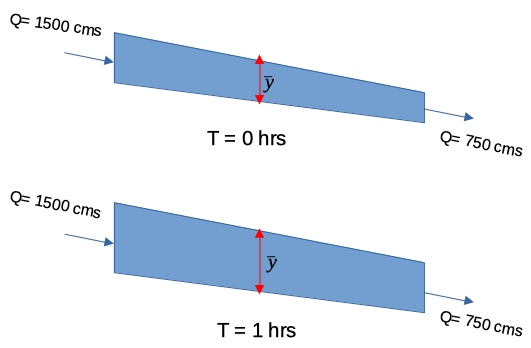
The river flow at an upstream gauging station is measured as 1500 $\frac{m^3}{sec}$, and at another gauging station 3 $km$ downstream, the discharge is measured as 750 $\frac{m^3}{sec}$ at the same moment in time. The channel is uniform, with a width of 300 $m$.
Determine:
- The rate of change in the average water surface elevation in meters per hour.
- Whether the stage (average water surface elevation) is rising or falling.
sketch(s) here
list known quantities
The problem statement supplies:
- Station 1 is upstream of station 2
- At station 1; $Q_1=~1500 \frac{m^3}{s}$,$x_1=0~m$,$T_1=300~m$
- At station 2; $Q_2=~750 \frac{m^3}{s}$,$x_2=3000~m$,$T_2=300~m$
list unknown quantities
The change in $y$, and the sign of the change.
governing principles
Here we apply continunity in a generalized structure:
$$( \frac{\partial y}{\partial t}) *T(y) + \frac{\partial Q}{\partial x} = 0$$Solution (step-by-step/computations)
So we will set-up the computations for this case
$\frac{\Delta WSE}{\Delta t} = \frac{\partial(y)}{\partial t} + \frac{\partial(z)}{\partial t}$
but $z$ is the channel bottom, which should be time invariant so
$\frac{\Delta WSE}{\Delta t} = \frac{\partial y}{\partial t}$
The spatial change in discharge is given in the problem so that
$\frac{\partial Q}{\partial x} = \frac{\Delta Q}{\Delta x} = \frac{Q_2 - Q_1}{x_2 - x_1}$
Now make the substitutions
$ \frac{\partial y}{\partial t} = \frac{(\frac{Q_1 - Q_2}{x_1 - x_2})}{T(y)}$
And script a solution
# script
Q1 = 1500
Q2 = 750
T1 = 300
T2 = 300
X1 = 0
X2 = 3000

DQDX = (Q2-Q1)/(X2-X1)
dydt = -DQDX/((T1+T2)*0.5)
if dydt > 0.0:
    print("WSE is changing at",dydt*3600,"meters per hour, and rising")
else:
    print("WSE is changing at",dydt*3600,"meters per hour, and falling")
discussion
- Direct application of conservation of mass.
- In this case we used the average topwidth to quantify the storage prism.
Problem 2
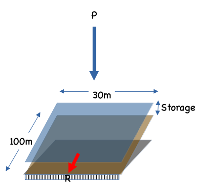
A paved parking lot section has a uniform slope over a length of 100 $m$ (in the flow direction) from the point of a drainage area divide to the inlet grate, which extends across the lot width of 30 $m$. Rainfall is occuring at a constant intensity of 100 $\frac{mm}{hr}$. The detention storage on the paved section is accumulating (increasing) at a rate of 60 $\frac{m^3}{hr}$
Determine:
- Runoff rate into the inlet grate (in $\frac{m^3}{sec}$)
sketch(s) here
list known quantities
- $P = 100~\frac{mm}{hr}$
- $S = 60~\frac{m^3}{hr}
- Geometry (on sketch)
list unknown quantities
- R
governing principles
- Conservation of mass $\dot I - \dot O = \frac{\Delta S}{\Delta t}$
# solution (step-by-step/computations)
P = 100*(1/1000) # mm/hr convert to m/hr
A = 100*30 # area m^2
Inflow = P*A
DsDt = 60 # m^3/hr
Outflow = Inflow - DsDt
print("Runoff =",round(Outflow,3)," m^3/hr")
discussion
Direct application of mass balance
Problem 3
A symmetric compound channel in overbank flow has a main channel with a bottom width of 30 $m$, side slopes of 1:1,and a flow depth of 3 $m$. The floodplains on either side of the main channel are 300 $m$ wide and flowing at a depth of 0.5 $m$. The mean velocity in the main channel is 1.5 $\frac{m}{sec}$ whereas the floodplain flow portion has a mean section velocity of 0.3 $\frac{m}{sec}$. The velocity variation within the main channel and floodplain subsections are assumed to be much smaller than the change in mean velocities between subsections.
Determine:
- The value of the kinetic energy correction coefficient $\alpha$
# sketch(s) here
# list known quantities
# list unknown quantities
# governing principles
# solution (step-by-step/computations)
amain=0.5*35+2.5*30+2.5*2.5
amain
afp = 300
qtotal = 1.5*amain+0.3*afp
Vs = qtotal/(amain+afp)
alpha = ((1.5**3)*amain+(0.3**3)*afp)/((amain+afp)*Vs**3)
print("Kinetic energy correction coefficient ",round(alpha,3))
# discussion
Problem 4
A bridge has cylindrical piers 1 $m$ in diameter and spaced 15 $m$ apart.
Downstream of the bridge, where the flow disturbance from the piers is no longer present, the flow depth is 2.9 $m$ and the mean velocity is 2.5 $\frac{m}{sec}$
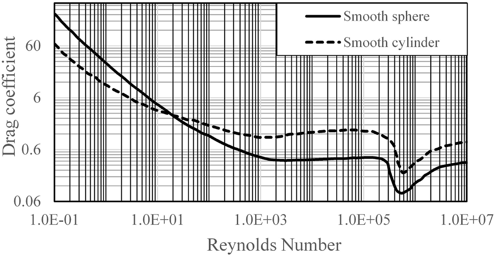
Figure 4 is a typical graph of drag coefficient for a single cylinder
Determine
- The Reynolds number for the flow described (use the flow depth as the characteristic length)
- The drag coefficient, $C_d$ for a cylinder at the computed Reynolds number
- The depth of flow upstream of the bridge
- The head loss caused by the piers
sketch(s) here
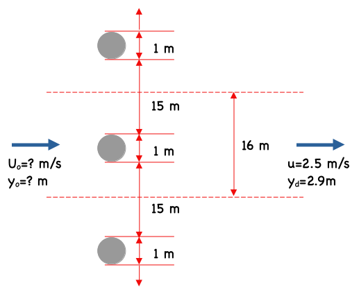
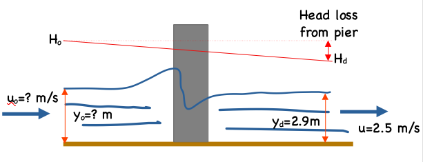
The sketch below ia a plan view of the described conditions, we will analyze a 16 meter wide portion of the flow field; total width is unknown, and we will assume the single pier estimate applies across entire width.
An elevation view sketch is below - showing the energy grade line (as a nice gradient, in actuality all the head loss will be quite near the pier.
list known quantities
- $y_d = 2.9$ meters
- $u_d = 2.5$ meters per second
- $D_{pier} = 1.0$ meter
- Pier array spacing is 15 meters
list unknown quantities
- $y_o = ?$ meters
- $u_o = ?$ meters per second
governing principles
- Continunity; will appear as specific discharge $\frac{Q}{width} = const.$
- Conservation of linear momentum
- Concept of drag force
Approach is use Continunity and Momentum to find the upstream depth and velocity, then use the energy equation to infer head loss.
## solution (step-by-step/computations)

# Material Properties
rho = 1000 #kg/m^3
mu = 0.001 #N-s/m^2
nu = 1e-06 #s/m^2
vd = 2.5 # downstream velocity
dchar = 2.9 # characteristic depth

## Reynolds number
def Re(v,d,nu):
    Re = v*d/nu
    return(Re)

print("Reynolds Number based on depth",round(Re(vd,dchar,nu),3))
## Discharge/unit width

q = vd*dchar

print("Specific discharge ",round(q,3)," m^2/sec")
Cd = 0.96 #look up in chart

def Fd(Cd,A,rho,V):
    Fd = 0.5*Cd*A*rho*V**2
    return(Fd)

print("Drag on Cylinder ",round(Fd(Cd,1*dchar,rho,vd),3)," Newtons")
Now some more analysis
First a control volume on a 16-meter wide portion of channel that encloses 1 pier (as in the plan view)
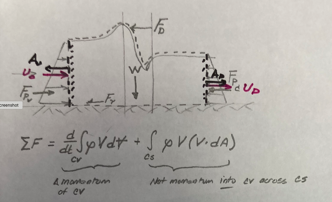
Now the force balance rendering

Next some algebra

We can probably switch back to code
W = 16 #m channel withn between equally spaced piers
g = 9.8 #m/s^2 our friend grabity
yd = 2.9 #m yes i know its the same as dchar, but dont want python equivalence here
ud = 2.5 # m/s
Cd = 0.96 # from above
Q = q*W
D = 1.0 # m diameter of a pier

#now a couple of fun shuns

def lhs(yu,yd,width,uu,Cd,gravity,diameter):
    term1 = (gravity*width*yu**2)/2
    term2 = (gravity*width*yd**2)/2
    term3 = (Cd*diameter*yu*uu**2)/2
    lhs = term1-term2-term3
    return(lhs)

def rhs(uu,ud,Q):
    rhs = (ud-uu)*Q
    return(rhs)

# check using

#print(lhs(2.92,yd,W,2.48,Cd,g,D))
#print(rhs(2.48,ud,Q))

# by brute force - guess yu, compute uu from Q supply to lhs,rhs when same have a solution print result

tolerance = 0.5
import math

yrange = [i/1000 for i in range(1000,10000)]
print("Depth (m) |","Velocity (m/s) |","Momentum Error ")
for irow in range(len(yrange)):
    yu = yrange[irow]
    uu = Q/(W*yu)
    test = lhs(yu,yd,W,uu,Cd,g,D)-rhs(uu,ud,Q)
    if abs(test) < tolerance:
        print(round(yu,3)," | ",round(uu,3),"  | ",round(lhs(yu,yd,W,uu,Cd,g,D)-rhs(uu,ud,Q),3))

#yrange
So by a brute force search, the following values are indicated
- $y_o = 2.924$
- $u_o = 2.479$
The momentum balance error is $-0.05$, if we wanted could jack the search a bit to get another digit maybe. But this is probably close enough.
Now finally determine the energy loss from
$$ y_o + \frac{u_o^2}{2g} = y_d + \frac{u_d^2}{2g} + \Delta H $$Solve for $\Delta H$
yu = 2.924
uu = 2.479
Eup = yu + (uu**2)/(2*g)
Edown = yd + (ud**2)/(2*g)
DeltaH = Eup - Edown
print("Head loss ",round(DeltaH,3)," meters")
discussion
This is just a fluid mechanics problem, to find the drag force impact on flow, then definition of head loss. Only hard part is finding Nemo ($C_d$)