Problem 1.
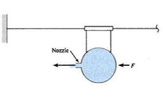
The figure is a schematic of a balloon rocket held in place by a force $F$.
The nozzle is a 0.8 $cm$ diameter tube, and an air jet exits the nozzle with a speed of 45 $m/s$ and a density of 1.2 $kg/m^3$.
Determine:
- The force $F$ needed to hold the balloon stationary.
# sketch here
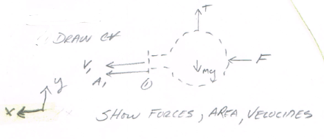
# list known quantities

# list unknown quantities
$F$
# governing principles
- Continunity
- Conservation of momentum; the linear type
# solution (step-by-step)
- Conservation-o-Momentum
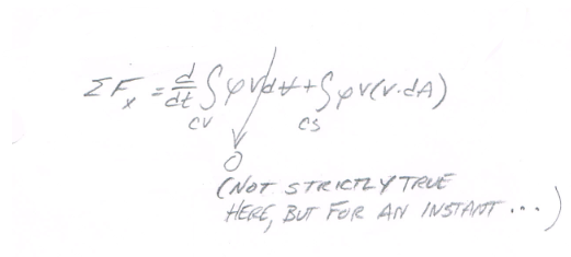
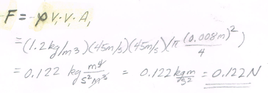
Then some algerbra
import math
rho = 1.2 #kg/m^3
v_i = 45 #m/sec
pie = math.pi
fore = math.sqrt(16)
diameter = 0.008 # meters
farce = rho*(v_i**2)*(pie*diameter**2/fore)
print("May the Force of :",round(farce,3),"N be with you!")
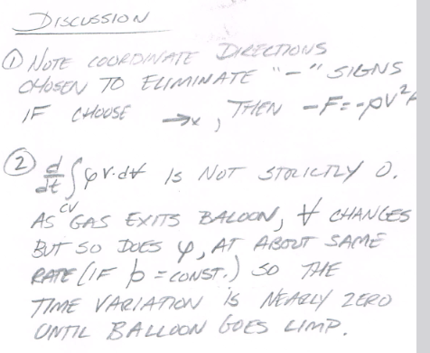
# discussion Other than the smartassery in the script above. Relative straight forward application of momentum. Obviously it only applies for a short time: from a solution circa 2014:
Problem 2.
Below is a schematic of an elbow fitting in a pipe system.
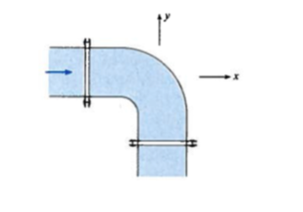
The gage pressure throughout the horizontal 90$^o$ bend (the elbow lies in the horizontal plane -- the figure is a plan view of the bend) is 300 $kPa$. The pipe diameter is 1 $m$ and the water (at 10 $^oC$) flow rate is 10 $m^3/s$
Determine:
- The $x-$component of force must be applied to the bend to hold in in place against the water action.
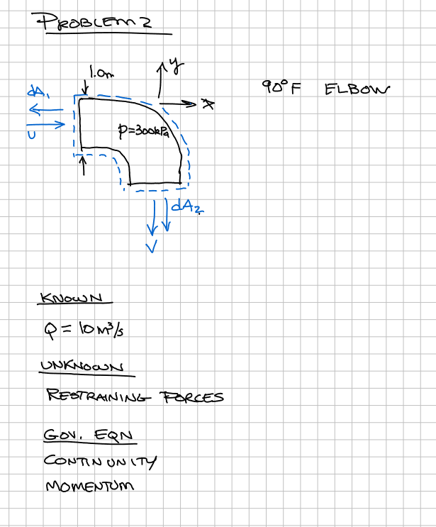
# sketch here
# list known quantities
Q, diameter, pressure, $\rho=1000$
# list unknown quantities
- $F_x$,$F_y$, Schrödinger's state.
# governing principles
- momentum, continunity
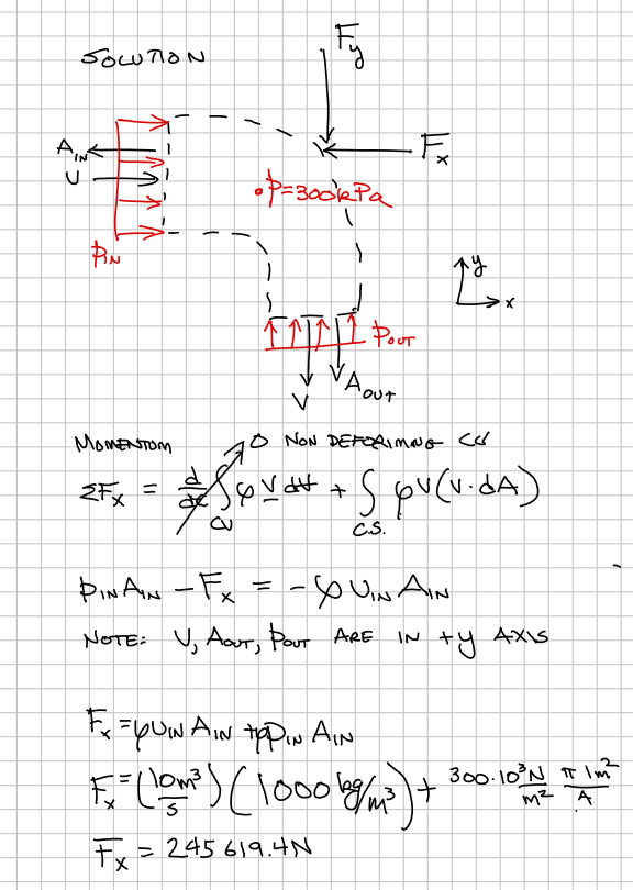
# solution (step-by-step)
rho = 1000 #kg/m^3
diameter = 1.0 #m
area = math.pi*diameter*diameter*0.25
flow = 10.0 #m^3/s given
pressure = 300e03 #Pa
u_in=flow/area
force_x=rho*(u_in*area)+(pressure*area)
print("Flow : ",round(flow,3),"m^3/s")
print("Velocity in : ",round(u_in,3),"m/s")
print("Force : ",round(force_x,1),"N to the LEFT")
# discussion
Linear momentum as defined by RTT
Problem 3.
Figure 2 is a schematic of a pumped-storage system. How much power must be supplied to the water by the pump (in kilowatts) to pump water at $0.085~m^3/s$ at 20$^o$C from the lower to the upper reservoir?
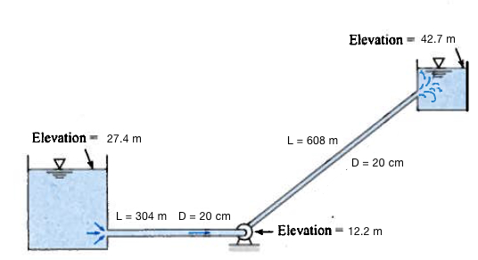
The head loss in the pipes is $h_l = 0.018 \frac{L}{D} \frac{V^2}{2g}$ , where $L$ is the length of the pipe in meters, and $D$ is the diameter of the pipe in meters.
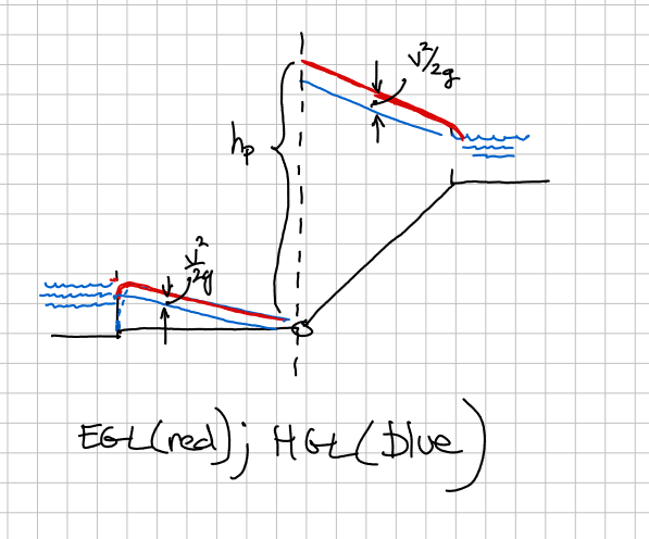
Sketch the HGL and EGL for the system.
# sketch here
# list known quantities
- Pool elevations
- Pipe lengths
- Pipe diameters
- $Q$
- Head loss function
# list unknown quantities
- Added head
- Power
- EGL/HGL
# governing principles
- Continuinty
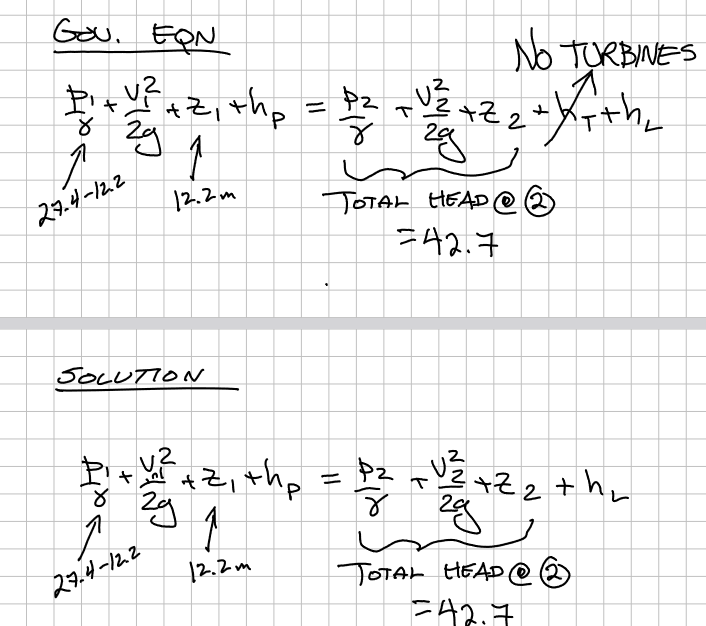
- Modified bernoulli
- Definition of flow work
# Solution
By hand
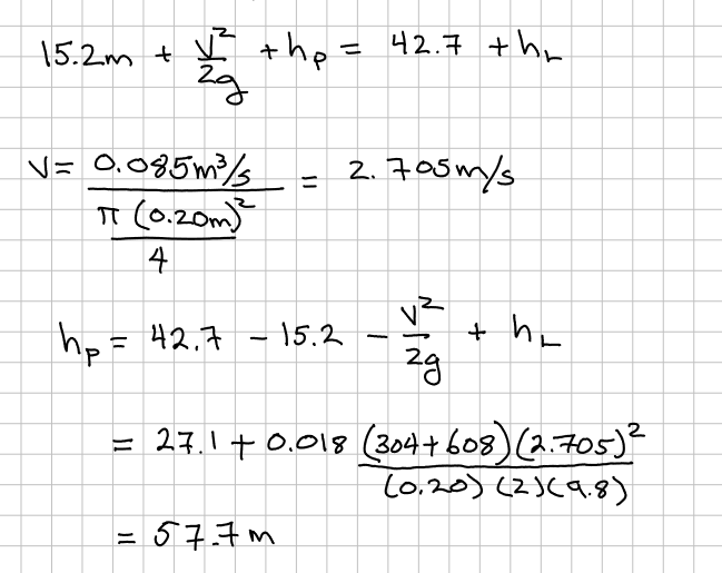
Using scripting language
# solution (step-by-step)
import math
flow = 0.085 #m^3/s
diameter = 0.20 #m
pie = math.pi
gee = 9.8 #m/s/s
#
area = (pie*diameter**2)/4.0
velocity = flow/area
# guillotine function (head loss)
def headloss(length,diameter,velocity,gee):
    headloss = (0.018*length*velocity**2)/(2*diameter*gee)
    return headloss
length = 304+608
pumphead = 42.7-15.2-(velocity**2)/(2*gee)+headloss(length,diameter,velocity,gee)
print("Added head from pump : ",round(pumphead,3)," meters at Q = :",flow," m3/sec")
rho = 1000 #kg/m^3
power = flow*rho*gee*pumphead
print("Power used :",round(power,3)," N-m/sec")
Hand drawn
# discussion
Straight forward application of energy equation. Note use of total head where possible - could have also used it at the left reservoir.
Problem 4.
Figure 1 is a schematic of a pipe with a series of holes used to sparge (introduce gas bubbles) gas into a larger volume.

The volumetric flow rate through each hole depends on the pressure difference across the hole and is given by $$Q = 0.67A_0(\frac{2 \Delta p}{\rho})^{1/2} $$ where $A_0$ is the area of the hole, $\Delta p$ is the pressure difference across the hole, and $\rho$ is the density of gas in the pipe. If the pipe is sufficiently large, the pressure will be uniform along the pipe.
A distribution pipe for air at 20$^o~C$ is 0.5 meters in diameter and 10 m long. The gage pressure in the pipe is 100 Pa. The pressure outside the pipe is atmospheric at 1 bar. The hole diameter is 2.5 cm, and there are 50 holes per meter length of pipe. The pressure is constant in the pipe.
Determine
- The velocity of air entering the pipe
# sketch here
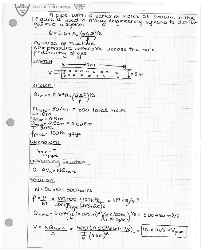
# discussion
A continunity, and PVNRT problem. Some geometry too